1. 퍼셉트론 (Perceptron)
두 종류의 클래스를 직선으로 분류하는 선형 분류기
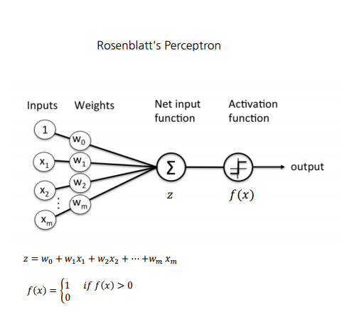
- 이진 분류만 가능
- 비선형 문제 못 품
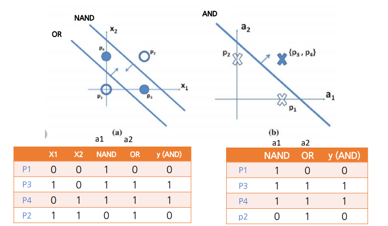
2. XOR 문제
-
퍼셉트론으로 XOR GATE 풀 수 X (비선형)
-> MLP 필요(퍼셉트론을 쌓아야 풀 수 있음) -
Layer를 쌓으면, 축이 바뀌면서(=문제가 바뀜) 해결 가능?
-
MLP를 학습 시킬 수 있는 방법이 X
-> 1st AI Winter
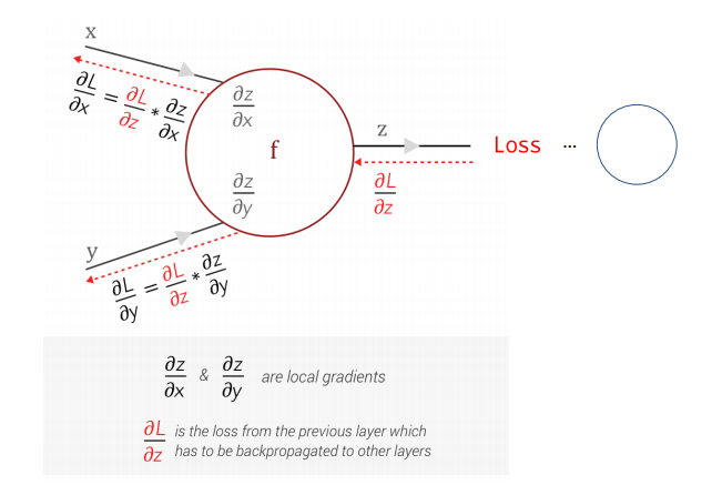
3. 오차 역전파(Backpropagation)
- MLP 학습시킬 수 있는 알고리즘
- 오차를 네트워크의 뒤로 전달하면서 가중치 갱신
1) 순전파
-
결과값 식을 가중치에 대해 편미분하면, 그 가중치가 결과에 얼마만큼 영향을 미치는지 알 수 있음
-
미분값 계산하여 저장
2) 역전파
- 임의의 한 노드에서의 미분값은, 바로 앞 노드에서 넘어오는 미분값에 로컬 미분값을 곱하는 것만으로 계산 가능
4. 기울기 소실(Gradient Vanishing)
깊은 신경망에서 입력층으로 갈수록 역전파 과정에서 미분값이 사라지면서 학습이 안되는 현상
- 원인: Sigmoid의 미분값이 곱해지면서 기울기가 0으로 사라짐
-> 2nd AI winter
5. Deep Learning
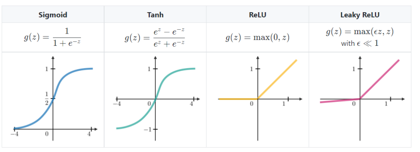
1) 활성화 함수
-> 주로 ReLU 함수 사용
2) 학습
-
학습율 조정
-
Noramalize
-
주로 미니 배치 사용
-
Optimizer: 경사 하강법
-
교차 검증
-
데이터 증강: 충분한 양의 데이터를 얻기 위함
-> 기존 데이터 변형, 생성 모델로 생성 -
Dropout(과적합 방지): 모델 학습에만 사용
-
규제: 과적합 해결 방법
-
가중치 초기화: Weight, Bias 설정
-
배치 정규화: 가중치의 초깃값에 상관업이 활성화값을 강제로 분포시킴
-> 미니배치별로 학습 바로 전/후에 정규화
6. 실습1
- Tensorflow 내 Keras 사용
- 뉴럴 네트워크 다중 선형회귀
1) 데이터 준비
import numpy as np
import pandas as pd
import matplotlib.pyplot as plt
import seaborn as sns
import tensorflow as tf

# tensorflow 버전: 2.14.0

!wget https://raw.githubusercontent.com/devdio/datasets/main/auto-mpg.csv

mpg = pd.read_csv('auto-mpg.csv', na_values=['?', '-']) # '?', '-' 는 결측치 처리 해라
df = mpg.copy()
df.columns = [ s.replace(' ','_') for s in df.columns ]
df.head() # 확인- horsepower가 왜 object형
->'?' 존재: csv 파일 읽을 때부터 결측치 처리해주기!
2) 테스트 데이터 분리
X = df.drop(['mpg','origin','car_name'], axis=1)
y = df['mpg']

from sklearn.model_selection import train_test_split

X_train, X_test, y_train, y_test = train_test_split(X, y, test_size=0.2, random_state=42)

X_train.shape, X_test.shape, y_train.shape, y_test.shape
3) 전처리
- 결측치 삭제
X_train = X_train.dropna()
y_train = y_train[X_train.index]

X_train.shape, y_train.shape- 스케일링
from sklearn.preprocessing import StandardScaler

scaler = StandardScaler()
X_train_s = scaler.fit_transform(X_train)

X_train_s

# y_train ndarray로
y_train = y_train.values
4) 모델 만들기
from tensorflow import keras
from keras import layers
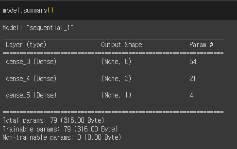
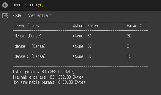
model = keras.Sequential([
layers.Dense(units=6, activation='relu', input_shape=(6,)),
layers.Dense(units=3, activation='relu'),
layers.Dense(units=1) # 출력층
])
model.summary()- 모델 컴파일
- 함수 결정
- 옵티마이저(어떤 경사하강법을 사용할건지)
- 매트릭스(MAE, MSE)
model.compile(
    loss='mse',
    optimizer='adam',
    metrics=['mse','mae']
)- 학습
EPOCHS = 80 # 반복 횟수
BATCH_SIZE = 16 # 데이터 크기

history = model.fit(
    X_train_s, y_train,
    batch_size = BATCH_SIZE,
    epochs = EPOCHS,
    verbose = 1
)
5) 평가
- 그래프
# 그래프
hist = history.history
epoch = history.epoch

plt.plot(epoch, hist['loss'], label='loss')
plt.show()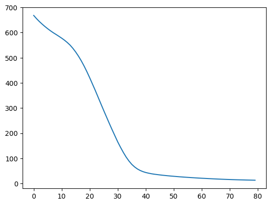
- 테스트 데이터 전처리
X_test.isna().sum()

X_test = X_test.dropna()
y_test = y[X_test.index] # X에서 결측치 제거했으니, y도 개수 맞춰주기

X_test.shape, y_test.shape # 확인

# 스케일링
X_test_s = scaler.transform(X_test)

y_pred = model.predict(X_test_s)

from sklearn.metrics import mean_squared_error
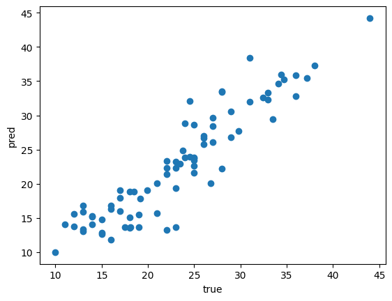
mean_squared_error(y_test, y_pred)- 위의 실행 결과가 좋은 값인지 그래프 그려서 확인
plt.scatter(y_test, y_pred)
plt.xlabel('true') # 정답
plt.ylabel('pred') # 예측
plt.show()
-> 좁게 모여있을수록 잘 예측한 것
7. 실습2
- 뉴럴 네트워크 이진 분류
- diabetes dataset
import numpy as np
import pandas as pd
import matplotlib.pyplot as plt
import seaborn as sns
import tensorflow as tf

!wget https://raw.githubusercontent.com/devdio/datasets/main/diabetes.csv
1) 데이터 준비
diabetes = pd.read_csv('diabetes.csv')
df = diabetes.copy()
df.head()
2) 테스트 데이터 분리
X = df.drop(['Outcome'], axis=1)
y = df['Outcome']

from sklearn.model_selection import train_test_split

X_train, X_test, y_train, y_test = train_test_split(X, y, test_size=0.2, random_state=42)

X_train.shape, X_test.shape, y_train.shape, y_test.shape
3) 전처리 - 이상치 처리 생략
# 스케일링
from sklearn.preprocessing import StandardScaler

scaler = StandardScaler()
X_train_s = scaler.fit_transform(X_train)

y_train = y_train.values
4) 모델 만들기
- feaure 수 확인
X_train_s.shape - 모델
# unit 수 증가 -> 모델 복잡 -> 과적합 가능성 증
from tensorflow import keras
from keras import layers

model = keras.Sequential([
    layers.Dense(units=6, activation='relu', input_shape=(8,)), # 1번째 layer
    layers.Dense(units=3, activation='relu'), # 2번째 layer
    layers.Dense(units=1, activation='sigmoid') # 출력층 - 이진분류: sigmoid 사용
])
5) 학습
- 컴파일
model.compile(
    loss='binary_crossentropy',
    optimizer='adam',
    metrics=['accuracy']
)- 학습
EPOCHS = 100
BATCH_SIZE = 16

history = model.fit(
    X_train_s, y_train,
    batch_size = BATCH_SIZE,
    epochs = EPOCHS,
    validation_split = 0.2, # validation 데이터 분리(0.2%)
    verbose = 1
)- 그래프
def plot_history(history):
    hist = pd.DataFrame(history.history)
    hist['epoch'] = history.epoch

    plt.figure(figsize=(16, 8))
    plt.subplot(1,2,1)
    plt.xlabel('epoch')
    plt.ylabel('loss')
    plt.plot(hist['epoch'], hist['loss'], label='train loss')
    plt.plot(hist['epoch'], hist['val_loss'], label='val oss')
    plt.legend()

    plt.subplot(1,2,2)
    plt.xlabel('epoch')
    plt.ylabel('accuracy')
    plt.plot(hist['epoch'], hist['accuracy'], label='train accuracy')
    plt.plot(hist['epoch'], hist['val_accuracy'], label='val accuracy')
    plt.legend()
plt.show() 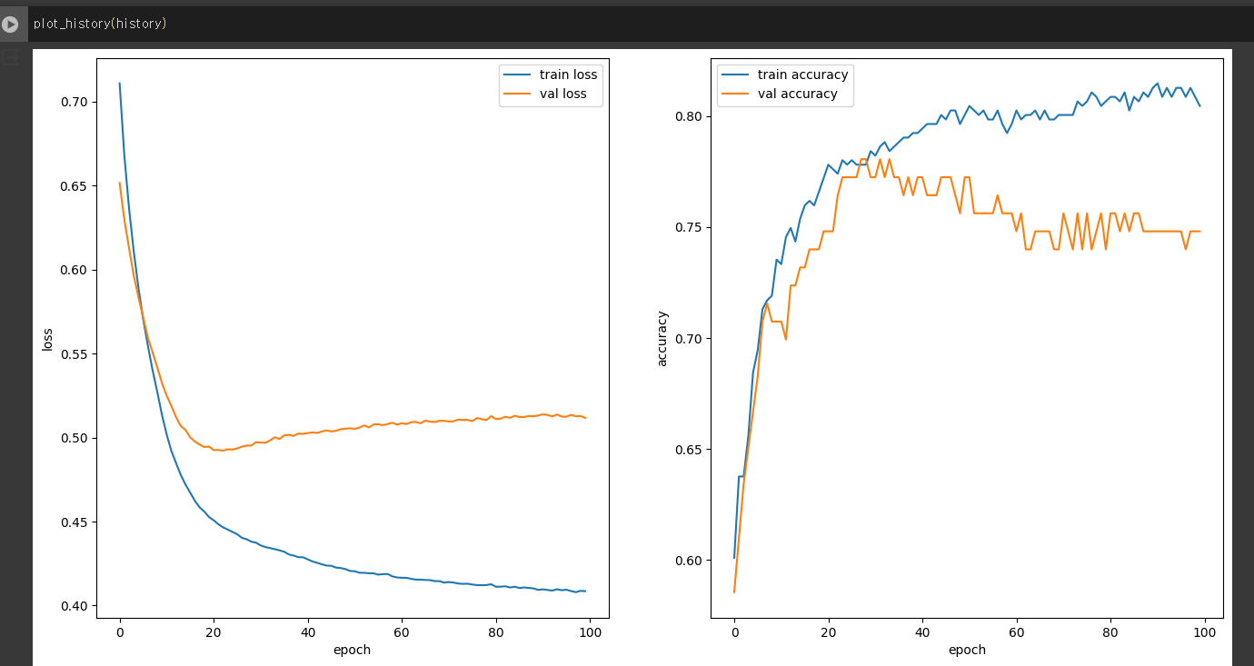
-> validation 데이터: 학습이 안되고 있음
6)평가
X_test_s = scaler.transform(X_test)
y_test = y_test.values # numpy로

y_pred = model.predict(X_test_s)
y_pred = y_pred.reshape(-1) # 1차원으로 바꾸기

y_pred = (y_pred > 0.5).astype('int') # True: 1, False:0- 정확도
from sklearn.metrics import accuracy_score,recall_score, precision_score

def print_metrics(y_test, y_pred):
  print(f'accuray: {accuracy_score(y_test, y_pred)}')
  print(f'recall: {recall_score(y_test, y_pred)}')
  print(f'precision: {precision_score(y_test, y_pred)}')

print_metrics(y_test, y_pred)
8. 실습3
-
뉴럴 네트워크 다중 분류
-
iris dataset
-
데이터 준비, 분리, 전처리 코드 생략
1) 레이블 인코딩, 원핫 인코딩
from sklearn.preprocessing import LabelEncoder

le = LabelEncoder()
y_train = le.fit_transform(y_train)

# 원핫 인코딩
from keras.utils import to_categorical

y_train_o = to_categorical(y_train)
2) 모델 만들기
from tensorflow import keras
from keras import layers

model = keras.Sequential([
    layers.Dense(units=6, activation='relu', input_shape=(4,)), # 1번째 layer
    layers.Dense(units=3, activation='relu'), # 2번째 layer
    layers.Dense(units=3, activation='softmax') # 출력층 - softmax 사용
])
3) 학습
# 컴파일
model.compile(
    loss='categorical_crossentropy',
    optimizer='adam',
    metrics=['accuracy']
)

EPOCHS = 200
BATCH_SIZE = 16

history = model.fit(
    X_train_s, y_train_o,
    batch_size = BATCH_SIZE,
    epochs = EPOCHS,
    validation_split = 0.2, # validation 데이터 분리(0.2%)
    verbose = 1
)
4) 평가
- 그래프: 코드는 실습2와 동일
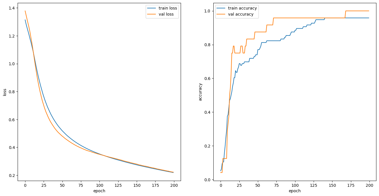
X_test_s = scaler.transform(X_test)
y_test = le.transform(y_test)

# 예측
y_pred = model.predict(X_test_s)

y_pred = np.argmax(y_pred,axis=1)- 정확도 확인
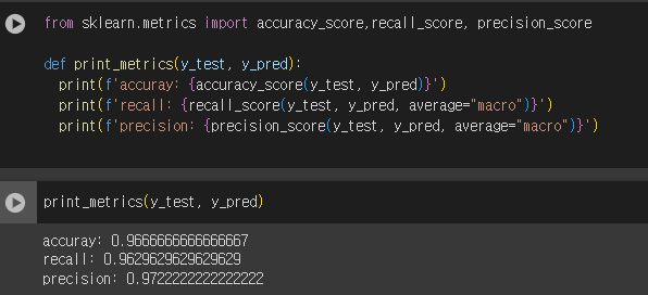
from sklearn.metrics import accuracy_score,recall_score, precision_score

def print_metrics(y_test, y_pred):
  print(f'accuray: {accuracy_score(y_test, y_pred)}')
  print(f'recall: {recall_score(y_test, y_pred, average="macro")}')
  print(f'precision: {precision_score(y_test, y_pred, average="macro")}')