[8일차] 1. 머신러닝 알고리즘

1. 의사 결정 나무(Decision Tree)

다른 지도 학습 기법들보다 성능이 떨어지지만, 구조가 단순하여 해석 용이

• 규제를 걸지 않으면 과적합 발생
• 선형, 비선형 관계 모두에 사용 가능
• 이상치의 영향 덜 받음 + 인코딩, 스케일링 필요X

<CART(Classification And Regression Tree) 알고리즘>

불순도가 감소하도록 노드를 분할하는 알고리즘

• 한 개의 노드는 이진 트리를 만든다

• gini : 불순도 점수
  sample : 노드에 속하는 샘플의 수
  value : 클래스별 샘플의 수
  class: 예측 클래스

• 불순도
  : 해당 범주 안에 서로 다른 데이터가 얼마나 섞여 있는지를 나타냄
  -> 각 노드의 분기 기준을 선택하기 위해 사용

• 정보 획득량
  : 하나의 질문에 의해서 감소되는 불순도의 정도

• 규제
  : 과적합을 막기 위해 필요
  • max_depth : 트리의 깊이를 제한
  • min_sample_split : 분기를 하기위한 최소한의 샘플 수
  • min_sample_leaf: 리프 노드 가지고 있어야 할 최소한의 샘플 수
  • max_leaf_nodes: 리프 노드의 최대수

• Feature Importance(변수 중요됴)
  : 어떤 변수가 가장 중요한지 나타내는 값으로, 불순도를 가장 크게 감소시킴

---

2. 의사 결정 나무 실습

• data: iris dataset

1) 필요 lib import

import numpy as np
import pandas as pd
import matplotlib.pyplot as plt
import seaborn as sns

import warnings
warnings.filterwarnings('ignore')

2) 데이터 준비

!wget https://archive.ics.uci.edu/static/public/53/iris.zip

!unzip iris.zip

• headr(첫 줄)에 데이터가 들어가있는 경우: header=None 설정

  • 열 이름 대신에 데이터가 들어있는 경우를 의미
  • 열 명 지정해주지 않으면, 0,1,..으로 출력됨

iris = pd.read_csv('iris.data', header=None)
iris.columns = ['sepal_length', 'sepal width','petal length','petal widtth','class'] # 열 이름 설
iris.shape

• 데이터 정보 확인

df = iris.copy()
df.head()

df.info()
df.describe().T 
df.isna().sum(axis=0) # nan 확인
df['class'].value_counts()

3) 테스트 데이터 분리

X = df.drop('class', axis=1)
y = df['class']

• X,y 나누지 않고 분리

from sklearn.model_selection import train_test_split

train_test_split(X, y, )
X, y = train_test_split(df, test_size=0.2, random_state=42) 
# 확인
X.shape, y.shape

• X,y 나눈 후 분리(위의 코드 실행했으면, 처음부터 다시 돌려야 함!)

from sklearn.model_selection import train_test_split

X_train, X_test, y_train, y_test = train_test_split(X, y, test_size=0.2, random_state=42)

X_train.shape, X_test.shape, y_train.shape, y_test.shape

4) 전처리

• 트리 알고리즘을 사용할 것이기 때문에 데이터 전처리X

5) 학습

• 학습시키기

columns = X_train.columns

X_train = X_train.values
y_train = y_train.values

from sklearn.tree import DecisionTreeClassifier

clf = DecisionTreeClassifier(random_state=42)
clf = clf.fit(X_train, y_train)

• 알고리즘 동작 그래프 확인

from sklearn.tree import plot_tree

plot_tree(clf, feature_names = columns, filled=True)
plt.show()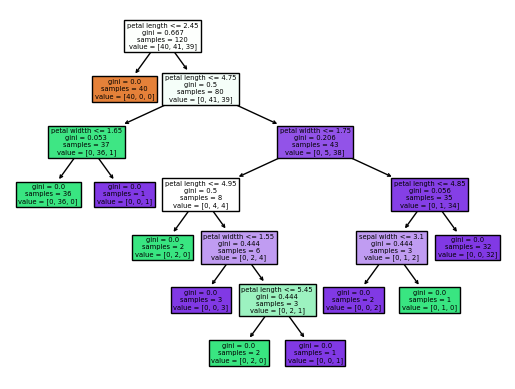

6) 평가

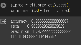
y_pred = clf.predict(X_test)

from sklearn.metrics import accuracy_score, recall_score, precision_score, f1_score

def print_metrics(y_test, y_pred):
  print(f'accuracy: {accuracy_score(y_test, y_pred)}')
  print(f'recall: {recall_score(y_test, y_pred, average="macro")}')
  print(f'precision: {precision_score(y_test, y_pred, average="macro")}')
  print(f'f1: {f1_score(y_test, y_pred, average="macro")}')

print_metrics(y_test, y_pred)

-> 정확도 1(과적합)

7) 튜닝

• max_depth 2로 조절하여 재학습

clf = DecisionTreeClassifier(max_depth=2, random_state=42)
clf = clf.fit(X_train, y_train)

from sklearn.tree import plot_tree

plot_tree(clf, feature_names = columns, filled=True)
plt.show()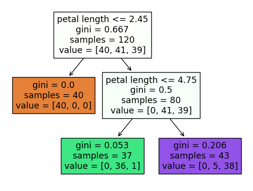

• 정확도
  

---

3. 앙상블(Ensemble Learning)

강력한 하나의 모델을 사용하기보다 약한 모델 여러 개를 조합하여 더 정확한 예측에 도움을 주는 방식

종류1) 보팅(Voting)

• 하드 보팅: 각 weak learner들의 예측 결과값을 바탕으로 다수결 투표하는 방식
• 소프트 보팅: weak learner들의 예측 확률값의 평균 or 가중치 합

종류2) 배깅(Bagging)

• Bootstrap Aggregating의 약자

• Bootstrap: 주어진 데이터셋에서 Random Sampling(중복 허용) 하여, 새로운 데이터셋을 만들어내는 것

• Random Forest: 결정 트리를 사용하는 배깅

종류3) 부스팅(Boosting)

• 앞의 분류기의 에러를 보완하는 약한 분류기를 차례로 연결하는 기법

• AdaBoost(아다 부스트)
  : 앞의 분류기에서 예측하지 못했던 데이터의 가중치를 높이는 방식

• Gradient Boost Machine(GBM)
  : 경사하강법 이용하여 가중치 업데이트

---

4. 랜덤포레스트 다중 분류 실습

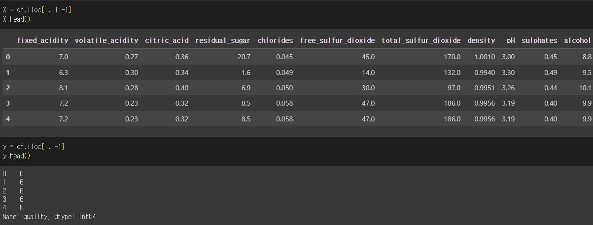
• data: 와인 품질 데이터셋

1) 데이터 준비

!wget https://raw.githubusercontent.com/devdio/datasets/main/winequalityN.csv

wine = pd.read_csv('winequalityN.csv')

• 데이터 확인

df = wine.copy()
df.head()
df.info()
df.describe().T

# 범주형 데이터 확인
df["type"].value_counts()
df["quality"].value_counts()
df["quality"].value_counts().sort_index() # 순서대로

2) 테스트 데이터 분리

• 타겟: quality
  

from sklearn.model_selection import train_test_split

X_train, X_test, y_train, y_test = train_test_split(
    X, y, stratify=y, test_size=0.2, random_state=0
)

3) 전처리

• quality값을 [3, 9] 에서 [0, 6]으로 변환
  

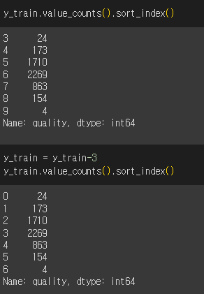
• 결측치 처리

X_train.isna().sum(axis=0) # 결측치 확인
X_train = X_train.dropna() # 결측치 제거
X_train.isna().sum(axis=0) # 다시 확인

• X_train shape에 맞게 y_train 수정

y_train = y_train[X_train.index]
y_train.shape # 확인

• 스케일링

# 데이터 표준화
from sklearn.preprocessing import StandardScaler

scaler = StandardScaler()
scaler.fit(X_train)
X_train_s = scaler.transform(X_train)

3) 학습 - RandomForest

• 베이스 모델

from sklearn.ensemble import RandomForestClassifier

clf = RandomForestClassifier(random_state=42)
clf.fit(X_train_s, y_train)

• test 데이터 전처리

# 결측치 삭제
X_test = X_test.dropna()
y_test = y_test[X_test.index]
X_test.shape, y_test.shape #  X_test와 y_test의 shape이 맞는지 확인

• y test 값 변경(train에서도 quality열에 3을 빼주었으니까)

y_test = y_test - 3
y_test.value_counts().sort_index()

• 스케일링

X_test_s = scaler.transform(X_test)

• 예측

y_pred = clf.predict(X_test_s)

• 정확도

from sklearn.metrics import (
    accuracy_score,
    f1_score,
    precision_score,
    recall_score
)

def print_metrics(y_test, y_pred):
    print("정확도:", accuracy_score(y_test, y_pred))
    print("정밀도:", precision_score(y_test, y_pred, average="macro"))
    print("재현율:", recall_score(y_test, y_pred, average="macro"))
    print("f1스코어:", f1_score(y_test, y_pred, average="macro"))

4) 튜닝

• GridSearchCV

from sklearn.model_selection import GridSearchCV

params = {
    "C": [0.1, 1],
    "gamma": [0.01, 0.1],
    "degree": [2,3],
    "kernel": ["linear", "poly", "rbf"]
}

grid_cv = GridSearchCV(SVC(), params, cv=5, refit=True, verbose=3) 
grid_cv.fit(X_train_s, y_train)

# best 파라미터 찾기
grid_cv.best_params_

# 위에서 구한 값으로 재학습
clf_best = SVC(C=1, degree=2, gamma= 0.1, kernel='rbf')
clf_best = clf.fit(X_train_s, y_train)

5) 다른 모델로 학습

• 서포터벡터모델

from sklearn.svm import SVC

clf = SVC(random_state = 42)
clf = clf.fit(X_train_s, y_train)

y_pred = clf.predict(X_test)
print_metrics(y_test, y_pred)

• 결정나무트리

from sklearn.tree import DecisionTreeClassifier

clf = DecisionTreeClassifier(random_state=42)
clf = clf.fit(X_train, y_train)

y_pred = clf.predict(X_test)
print_metrics(y_test, y_pred)