Dynamic Programming(이하 DP)는 Markov Decision Process(이하 MDP)의 model이 완벽하게 주어졌을 때 최적의 policy를 찾게해주는 방법이다.

단, 2가지의 조건 즉 제약이 따르는데
1. the assumption of a perfect model
2. great computational expense 이 해당된다.

그래서 이러한 제약 조건들 때문에 이후에 나오는 방법들은 computation이 작거나 perfect model을 모른다는 가정하에 DP와 유사한 성능을 내는 것을 목표로 한다.

Notation을 한번 더 짚고 넘어가면 현재의 MDP는 finite MDP라는 조건에 해당한다.
여기서 finite가 의미하는 것은 MDP를 구성하는 state, action, reward set이 finite하다는 것을 의미한다.
infinite으로의 확장은 뒤에 나오니 우선은 작은 문제들을 풀고 후에 더 큰 문제들을 푸는 방향으로 진행이 된다.
Notation은 아래와 같다.

state : $S$
action : $A$
reward : $R$
state transition probability : $p(s^,,r|s,a)$
state + termination state : $S^+$

state가 infinite 즉 continuous한 경우는 continuous한 값들을 quantize 즉 양자화하여 approximate하는 방법으로 environment를 구하고 이를 토대로 finite-state DP method에 적용하는 방법으로 하는데 이러한 방법은 뒤의 chapter 9에서 다룰 예정이다.

먼저 good policy를 찾는데에 기준이 필요한데 이는 chapter 3에 나온 Bellman optimality equation을 통해 알 수 있다.
$v_*(s) = max_aE[R_{t+1}+\gamma v_*(S_{t+1})|S_t=s,A_t=a] = max_a\sum_{s^,,r}p(s^,,r|s,a)[r+\gamma v_*(s^,)]$
$q_*(s,a) = E[R_{t+1}+\gamma max_{a^,}q_*(S_{t+1},a^,)|S_t=s,A_t=a] = \sum_{s^,,r}p(s^,,r|s,a)[r+\gamma max_{a^,}q_*(s^,,a^,)]$
for all $s$ in $S$, $a$ in $A$ and $s^,$ in $S^+$

즉 Bellman optimality equation의 해가 곧 optimal policy가 되므로 가능한 이와 유사한 policy를 찾는다!

4.1 Policy Evaluation (Prediction)

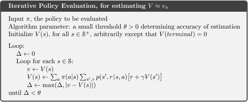
how to compute the state-value function $v_\pi$ 를 policy evaluation이라고 한다.
또 이러한 policy evaluation을 prediction problem이라고도 한다.

Bellman value function을 먼저 써보면 아래와 같다.
$v_\pi(s)=E_\pi[G_t|S_t=s]=E_\pi[R_{t+1}+\gamma G_{t+1}|S_t=s]=E_\pi[R_{t+1}+\gamma v_\pi(S_{t+1})|S_t=s]=\sum_a\pi(a|s)\sum_{s^,,r}p(s^,,r|s,a)[r+\gamma v_\pi(s^,)]$

이때 위의 연립 방정식의 해는(s가 S의 원소들에 해당하므로 연립방정식으로 나온다) iteration방법으로 구할 수 있다.
By jacobi iteration, gauss-seidel iteration
$v_{k+1}(s)=E_\pi[R_{t+1}+\gamma v_k(S_{t+1})|S_t=s]=\sum_a\pi(a|s)\sum_{s^,,r}p(s^,,r|s,a)[r+\gamma v_k(s^,)]$

이러한 방법으로 구하는 것을 iterative policy evaluation이라고 한다.
그리고 이러한 방법으로 한 번 $v(s)$의 값이 update되는 것을 expected update라고 한다.
이때 k+1과 k step의 $v(s)$값들의 집합이 있어야 하므로 메모리가 필요하며 완전히 수렴하는 것 보다 $max_{s in S}[v_{k+1}(s)-v_k(s)]$가 특정 값보다 작아지면 계산을 멈추는 방법으로 진행된다.

Example 4.1로는 grid world가 나온다.

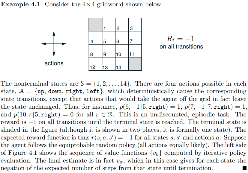
문제는 위와 같고 해당 문제를 구현한 코드 링크를 아래에 남긴다.
https://github.com/han811/sutton_rl_book/tree/main/chapter4_DP

gauss-seidel iteration의 수렴조건은 $Ax=b$ 라는 linear equation이 있을 때 행렬$A$가 diagonal dominant하면 된다.
증명은
$x_i=-\frac{1}{A_{ii}}(-b_i+\sum_{i!=j}A_{ij}x_j)$
$x_i^{k+1}=-\frac{1}{A_{ii}}(-b_i+\sum_{i!=j}A_{ij}x_j^{k})$
$e_i^{k+1}=-\frac{1}{A_{ii}}(\sum_{i!=j}A_{ij}e_j^{k})$
이때 diagonal dominant 조건인 $|A_{ii}|>\sum_{i!=j}|A_{ij}|$ 가 만족되면 오차는 계속 작아지므로 수렴함이 증명된다.

4.2 Policy Improvement

자 이제 policy에 대한 value function값과 action-value function값을 알고있으니 policy를 어떻게 개선할지에 대해 알아보자.
기준은 현재의 policy $\pi$와 다른 action을 취하는 새로운 policy $\pi^,$에 대하여 action-value function값이 더 커지는 지를 보면 된다.
이를 policy improvement라고 한다.

식으로 표현해보면
$q_\pi(s,a)=E[R_{t+1}+\gamma v_\pi(S_{t+1})|S_t=s, A_t=a]=\sum_{s^,,r}p(s^,,r|s,a)[r+\gamma v_\pi(s^,)]$에 대하여
$q_\pi(s,a)>=v_\pi(s)$ 즉 $q_\pi(s,\pi^,(s))>=v_\pi(s)$이 만족한다면
$v_{\pi^,}(s)>=v_\pi(s)$가 만족된다로 표현된다.

이에 대한 증명은 적기가 너무 힘들어서 책의 증명을 첨부한다.

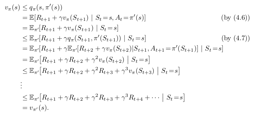
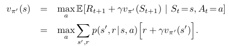
즉 아래의 식을 만족하는 새 policy $\pi^,$를 매번 구한다.

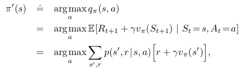
이때 어느 순간 새로운 policy를 구하여도 기존의 policy와 같은 상황이 생기는데 그러한 경우 optimal policy로 수렴한 것이다.
즉 다음의 Bellman optimality equation이 구하여 진다.

지금까지는 policy가 deterministic 하였다.
즉 s에서 넌 무조건 a라는 행동만 해! 인데 이러한 deteministic policy가 stochastic policy로 확장 될 수 있다.
뒤에서 더 다루게 되며 생각보다 쉽게 확장된다고 한다.
concept만 알아보면 결국 deterministic하게 policy를 정하였을 때 가장 높은 가치를 지니는 policy로 확률이 모일 때까지 돌린다는 것 같다.

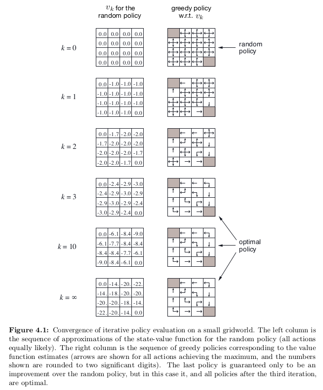
위는 example 4.1의 policy improvement 과정이다.
얘는 쉬운 문제여서 한번만 improvement해도 optimal policy가 구해진다.

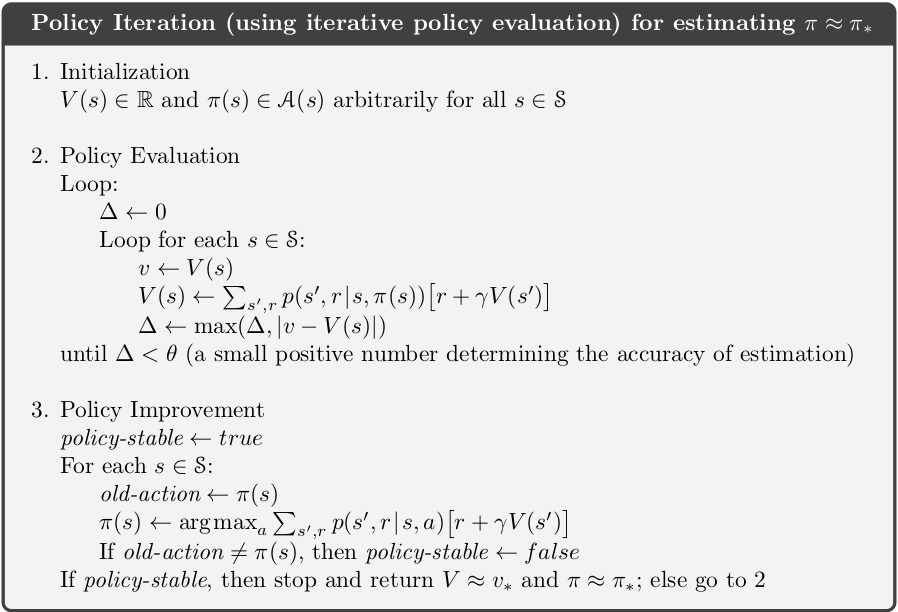
4.3 Policy Iteration

위에서 말했던 policy evaluation과 policy improvement를 반복해서 하는 것을 말한다.
즉 둘을 결합하여 optimal policy를 찾는 과정을 policy iteration이라고 한다.
pseudo-code는 아래와 같다.

Example 4.2로는 Jack's Car Rental 문제가 나온다.

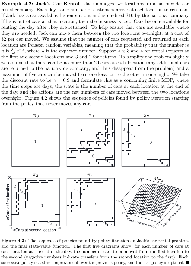
이 문제도 어려운 문제가 아니어서 생각보다 몇번의 iteration만으로 수렴한다.
https://github.com/han811/sutton_rl_book/tree/main/chapter4_DP

4.4 Value Iteration

그런데 매번 policy evaluation을 수렴할 때까지 하는 것은 많은 computation을 필요로한다.
그래서 figure 4.1을 보게 되면 policy evaluation을 수렴할 때까지 하지 않아도 policy improvement를 하는데 문제가 없는 경우를 볼 수 있다.
그래서 나온 idea가 policy evaluation을 할때 expected update를 한번만 진행하고 policy improvement를 진행하는 방안을 제시하며 이것이 value iteration이다.
pseudo-code로는 아래와 같다.

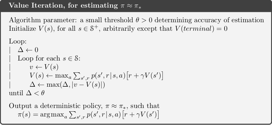
코드를 보면 $\theta$를 기준으로 evaluation이 결정되는데 value iteration은 이 값이 굉장히 커 loop가 한번만 돈다고 보면 되고 이 threshold값을 적절히 조절함으로써 evaluation에서 소모되는 computation을 절충하여 나간다.

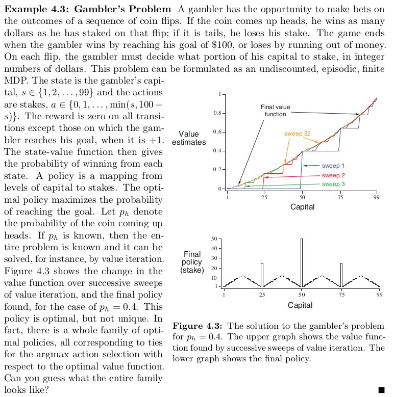
위의 결과를 보면 확실히 그래프에도 sweep 즉 evaluation loop가 적어도 수렴하며 수렴속도가 빠른걸 볼 수 있다.
https://github.com/han811/sutton_rl_book/tree/main/chapter4_DP

[Exercise 4.1]

In Example 4.1, if $\pi$ is the equiprobable random policy, what is $q_\pi(11, down)$?
What is $q_\pi(7, down)$?

sol)
$q_\pi(11, down)=-1+v_\pi(T)=-1+0=-1$
$q_\pi(7, down)=-1+v_\pi(11)=-1+(-14)=-15$

[Exercise 4.2]

In Example 4.1, suppose a new state 15 is added to the gridworld just below
state 13, and its actions, left, up, right, and down, take the agent to states 12, 13, 14, and 15, respectively.
Assume that the transitions from the original states are unchanged.
What, then, is $v_\pi(15)$ for the equiprobable random policy?
Now suppose the dynamics of state 13 are also changed, such that action down from state 13 takes the agent to the new state 15.
What is $v_\pi(15)$ for the equiprobable random policy in this case?

sol)
$v_\pi(15)=-1+0.25(-20-22-14+v_\pi(15))=-15+0.25v_\pi(15)$
따라서 $v_\pi(15)=-15/0.75=-20$

[Exercise 4.3]

What are the equations analogous to (4.3), (4.4), and (4.5) for the action-
value function $q_\pi$ and its successive approximation by a sequence of functions $q_0, q_1, q_2, ...$?

sol)
$q_\pi(s,a)=E_\pi[G_t|S_t=s,A_t=a]=E_\pi[R_{t+1}+\gamma G_{t+1}|S_t=s,A_t=a]=E_\pi[R_{t+1}+\gamma \sum_{s^,,a^,}q_\pi(s^,,a^,)|S_t=s,A_t=a]=\sum_{s^,,r}p(s^,,r|s,a)[r+\gamma\sum_{a^,}\pi(a^,|s^,)q_\pi(s^,,a^,)]$

$q_{k+1}(s,a)=E_\pi[R_{t+1}+\gamma G_{t+1}|S_t=s,A_t=a]=\sum_{s^,,r}p(s^,,r|s,a)[r+\gamma\sum_{a^,}\pi(a^,|s^,)q_k(s^,,a^,)]$

[Exercise 4.4]

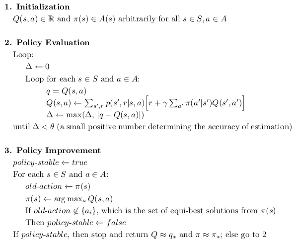
The policy iteration algorithm on page 80 has a subtle bug in that it may
never terminate if the policy continually switches between two or more policies that are equally good.
This is ok for pedagogy, but not for actual use.
Modify the pseudocode so that convergence is guaranteed.

sol)
step3에서 Policy Improvement할 때, If $old-action != \pi(s)$, then ...... 부분을 If old-action not in ${a_i}$, which is the all equi-best solutions from $\pi(s)$, ...... 으로 바꾸어 주면 된다.
즉 해당 policy와 같은 가치를 가지면 될 뿐 꼭 같은 policy일 필요는 없다.

[Exercise 4.5]

How would policy iteration be defined for action values?
Give a complete algorithm for computing $q_*$, analogous to that on page 80 for computing $v_*$.
Please pay special attention to this exercise, because the ideas involved will be used throughout the rest of the book.

sol)

[Exercise 4.6]

Suppose you are restricted to considering only policies that are $\epsilon$-soft, meaning that the probability of selecting each action in each state, s, is at least $\epsilon/|A(s)|$.
Describe qualitatively the changes that would be required in each of the steps 3, 2, and 1, in that order, of the policy iteration algorithm for $v_*$ on page 80.

sol)
step 1의 경우 policy $\pi$가 soft-$\epsilon$ 방법으로 변형되어야 한다.
step 2의 경우 threshold $\theta$가 soft-$\epsilon$ 방법으로 변형되어야 한다.
step 3의 경우 policy가 stable하다는 기준이 policy를 더 이상 explore하지 않는 것을 기준으로 해야한다.

[Exercise 4.7]

https://github.com/han811/sutton_rl_book/tree/main/chapter4_DP
[아직 미완성]

[Exercise 4.8]

Why does the optimal policy for the gambler’s problem have such a curious form?
In particular, for capital of 50 it bets it all on one flip, but for capital of 51 it does not.
Why is this a good policy?

sol)
50일 때는 바로 이길 수 있는 확률이 커서 풀 베팅을 하고 51일 때는 풀베팅보다 조금씩 더 돈을 얻어서 바로 이길 수 있는 확률이 커지도록 하는 것이 효과적이다.
즉 한번에 이길 수 있는 확률을 키우는 것도 있지만 져도 덜 피해보도록 학습이 이루어진다고 볼 수 있다.
아직 정확한 이해가 부족하여 이 부분 정답은 추후 보충해야겠다.

[Exercise 4.9]

https://github.com/han811/sutton_rl_book/tree/main/chapter4_DP
[아직 미완성]

[Exercise 4.10]

What is the analog of the value iteration update (4.10) for action values, $q_{k+1}(s,a)$?

sol)
$q_{k+1}(s,a)=E[R_{t+1}+max_{a^,}\gamma q_k(s^,,a^,)]=\sum_{s^,,r}p(s^,,r|s,a)[r+max_{a^,}\gamma q_k(s^,,a^,)]$