3.2 Monte Carlo(MC)

How can we get $Q^*$?

We have learned how to calculate maximum value of state value function by optimal policy. If the $Q^*$ is given, what we need to do is just find the policy maximizing $Q^*$. But, how can we get $Q^*$?

Actually, we cannot get $Q^*$ directly. We believe that if we train the agent with $\epsilon$-greedy, its action value function will get closer to $Q^*$. It may not be the best policy. But we believe it’s performance may be good enough. After training, we test the agent with greedy action(not $\epsilon$-greedy!!)

Monte Carlo : a method of getting $Q^*$

Recall expectation function :

The Monte Carlo method operates under the law of large numbers, asserting that as (N) increases, the approximated value in the equation above converges to the actual expectation.

Applying this method, we can express action value function in a different way.
$Q(s_t, a_t) \approx \frac {1}{N} \sum\limits_{i=1}^N G_t^{(i)}$
In this approximation, $G_t^{(i)}$ follows the probability distribution($p(s_{t+1}, a_{t+1},…|s_t, a_t)$).

Let’s get idea by reviewing Q-learning!

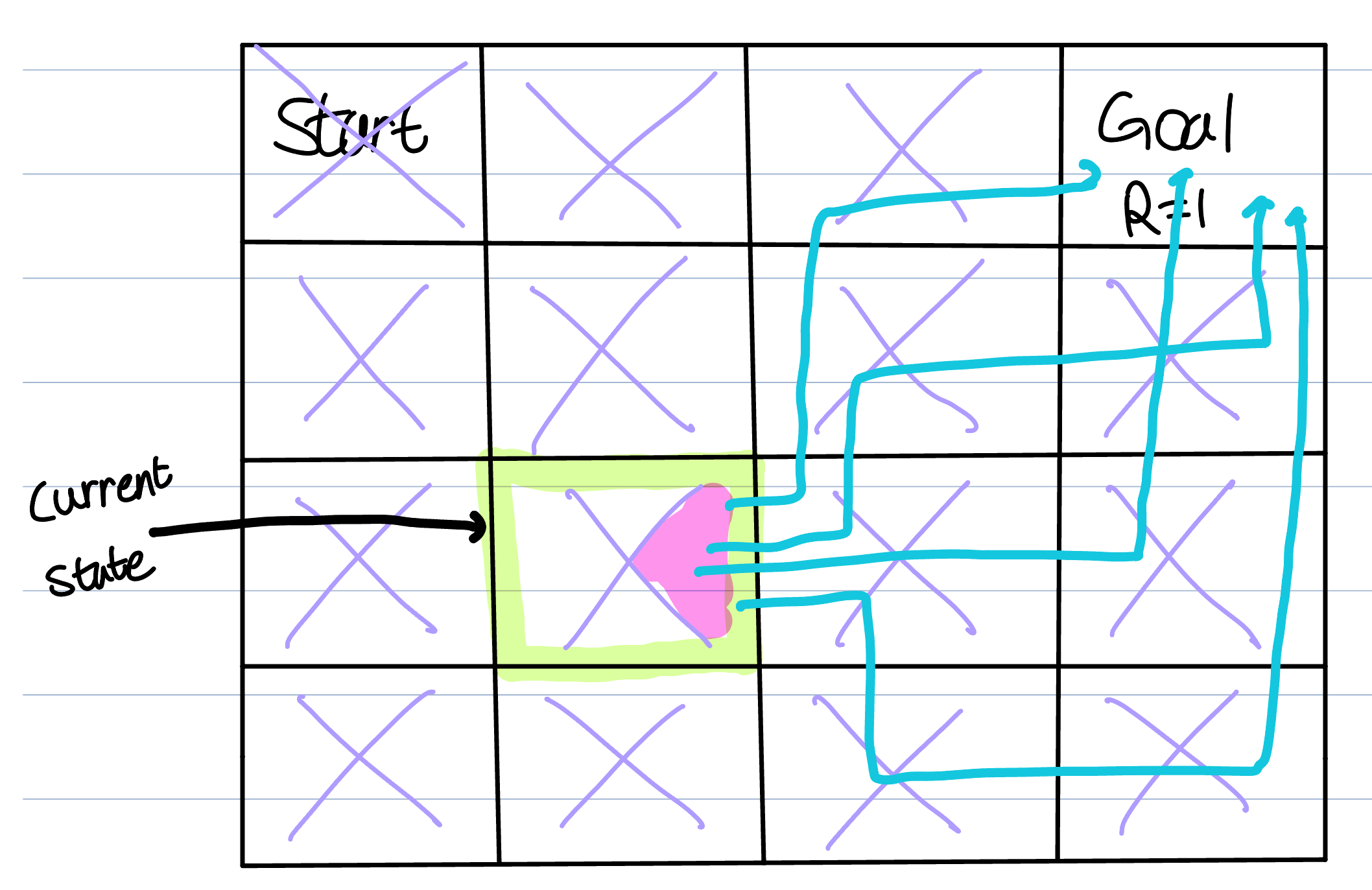
Let’s assume we want to evaluate $Q(s_t,a_t)$ at ‘right’ action(pink area). Initially, the agent explores all possible routes to reach the goal (this includes paths not marked in the given figure). The more paths the agent explores, the closer the approximation becomes to the original equation. However, it takes too much time. But we have to know the idea.

As the agent undergoes numerous episodes using epsilon-greedy, both Q and p improve. We train the agent until Q and p are sufficiently close to $Q^*$ and the optimal policy, respectively. Moreover, as the agent explores more possible routes, its understanding of the probability distribution becomes more comprehensive.