F-Divergence

두 개의 distribution $p, q$가 주어졌을 때 f-divergence는 다음과 같이 정의 된다.

• $D_f(p, q)=E_{\mathbf{x}\sim q}[f(\frac{p(\mathbf{x})}{q(\mathbf{x})})]$, $f$는 $f(1)=0$ 인 convex, semicontinous function

$f(1)=0$ 이기 때문에 jenson's inequality를 이용하면 $f$는 항상 non-negative function인 것을 알 수 있다. (증명은 생략) KL divergence도 f-divergece의 일종으로, $f(u)=u\log u$ 인 f-divergence이다.

Train with F-Divergence

$p_{data}, p_\theta$가 주어졌을 때, f-divergece는 아래와 같을 수 있다.

• $D_f(p_\theta,p_{data})=E_{\mathbf{x}\sim p_{data}}[f(\frac{p_\theta(\mathbf{x})}{p_{data}(\mathbf{x})})]$
• $D_f(p_{data},p_\theta)=E_{\mathbf{x}\sim p_\theta}[f(\frac{p_{data}(\mathbf{x})}{p_\theta(\mathbf{x})})]$

두 경우 모두 두 distribution의 ratio 즉, probaility 계산을 요구한다. likelihood free 가 되려면, train objective는 오직 samples만 이용해서 구할 수 있어야한다.

Fenchel Conjugate

Fenchel conjugate를 이용하면 samples만 이용하여 구할수 있는 trainig objective를 만들 수 있다. 어떤 convex function의 conjugate는 다음과 같이 정의될 수 있다.

• $f^*(t)=\underset{u\in\mathrm{dom_f}}{\sup}(ut-f(u))$, $\mathrm{dom_f}$는 $f$의 정의역.

또한 conjugate의 conjugate는 다음과 같이 구할 수 있다.

• $f^{**}(u)=\underset{t\in\mathrm{dom}_{f^*}}{\sup}(tu-f^*(t))$

$f$가 convex이면서 lower semicontinuos이면 $f^{**}=f$인 것이 알려져 있다. 이를 활용하면 아래와 같은 lower bound를 구할 수 있다.

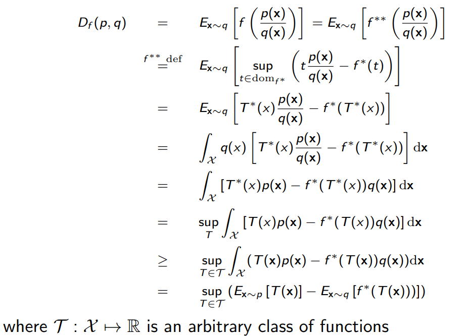
위 식 역시 likelihood free 인 것을 볼 수 있다.

F-GAN

이제 f-divergence를 이용한 GAN의 objective를 다음과 같은 lower bound를 이용하여 구할 수 있다.

• lower bound: $D_f(p,q)=\ge\underset{T\in\mathcal{T}}{\sup}(E_{\mathbf{x}\sim p}[T(\mathbf{x})]-E_{\mathbf{x}\sim q}[f^*(T(\mathbf{x}))])$
• $p=p_{data}$, $q=p_G$
• parameterize $T$ by $\phi$, $G$ by $\theta$
• f-GAN objective: $\underset{\theta}{\min}\underset{\phi}{\max}F(\theta,\phi)=E_{\mathbf{x}\sim p_{data}}[T_\phi(\mathbf{x})]-E_{\mathbf{x}\sim p_{G_\theta}}[f^*(T_\phi(\mathbf{x}))]$

이제 아무 f-divergence를 가지고 GAN을 training 할 수 있다.

Wassertstein GAN(WGAN)

Wassertstein GAN의 핵심 아이디어는 $p$ (true data distribution) 과 $q$ (generative data distribution) 이 smoothly change 하며 닮도록 하자는 것이다. 아래는 wassertstein distance에 대한 정의이다.

• $D_w(p,q)=\underset{\gamma\in\Pi(p,q)}{\inf}E_{(\mathbf{x,y})\sim\gamma}[||\mathbf{x-y||_1}]$, $\Pi(p,q)$는 모든 $\mathbf{x,y}$의 joint distribution을 갖고 있음.

위 식은 kantorovich-rubinstein duality로 다음과 같이 표현 가능하다.

• $D_w(p,q)=\underset{||f||_L\le1}{\sup}E_{\mathbf{x}\sim p}[f(\mathbf{x})] - E_{\mathbf{x}\sim q}[f(\mathbf{x})]$
  $||f||_L\le1$은 $f(\mathbf{x)}$ 의 Lipschitz constant가 1이라는 것을 의미.
  $\forall\mathbf{x,y}:|f(\mathbf{x})-f(\mathbf{y})|\le||\mathbf{x-y||_1}$

Lipschitz constant가 1 이하라는 것은 함수의 변화가 매우 빠르지 않다는 것을 의미한다.

$D_\phi(\mathbf{x})$를 discriminator, $G_\theta(\mathbf{x})$를 generator로 한 WGAN의 objective function은 아래와 같다.

• $\underset{\theta}{\min}\underset{\phi}{\max}E_{\mathbf{x}\sim p_{data}}[D_\phi(\mathbf{x})]-E_{\mathbf{z}\sim p(\mathbf{z})}[D_\phi(G_\theta(\mathbf{z}))]$

보통 $D_\phi(\mathbf{x})$의 Lipschitzness는 weight clipping이나 $\nabla_\mathbf{x}D_\phi(\mathbf{x})$의 gradient penalty를 통해 이루어진다. WGAN은 더 stable한 training이 가능하며, mode collapse 가능성이 비교적 낮다.

Inferring Latent Representation in GNAs(BiGAN)

BiGAN은 $\mathbf{x}$의 latent representation을 얻기 위해 encoder model을 추가한 형태의 GAN이다.

discriminator의 목표는 $\mathbf{z},G(\mathbf{z})$와 $E(\mathbf{x}), \mathbf{x}$ 사이의 two-sample test objective를 최대화 하는 것이다. 즉 $\mathbf{z}, E(\mathbf{x})$를 잘 구별하고, $G(\mathbf{z}), \mathbf{x}$를 잘 구별하는 것이다.

학습이 끝나고 나면 encoder model $E$를 가지고 data의 latent representation을 쉽게 얻을 수 있다.

Reference

cs236 Lecture 10