Parameterizing Probaility Distribution

Probaility는 다음과 같은 특징을 가진다.

• non-negative: $p(\mathbf{x})\ge0$
• sum-to-one: $\sum_\mathbf{x}p(\mathbf{x})=1$ or $\int p(\mathbf{x})d\mathbf{x}$

일반적으로 non-negative 특징을 만족시키기는 어렵지 않다. (exponetial function, square function 등을 이용) 그러나 모든 probability의 합이 1이 되도록 모델링하는 것은 꽤나 어려운 일이다.

sum-to-one을 해결하기 위한 방법으로 normalizing 방법을 생각 할 수 있다.

• $p_{\theta}(\mathbf{x})=\frac{1}{Z(\theta)}g_\theta(\mathbf{x})=\frac{1}{\int g_\theta(\mathbf{x})d\mathbf{x})}g_\theta(\mathbf{x})=\frac{1}{\mathrm{Volume(g_\theta)}}g_\theta(\mathbf{x})$

위 식에서 $Z(\theta)$를 normalize constant로 볼 수 있다. 위 식에 따르면, probability를 구하기 위해서는 $g_\theta$의 integral을 구해야한다. 따라서 $g_\theta$는 analytical integration이 되면 좋다. analytical integration이 되도록 $g_\theta$를 설정한 대표적인 예시가 Exponential family distributions 이다.(Normal distributnion, Poisson distribution 등) 그러나 이는 꽤 큰 제약 사항으로 모델의 자유도를 떨어뜨린다.

Energy-based Model

다음은 energy-based model의 probability 식이다.

• $p_\theta(\mathbf{x})=\frac{1}{\int \exp(f_\theta(\mathbf{x}))d\mathbf{x}}\exp(f_\theta(\mathbf{x}))=\frac{1}{Z(\theta)}\exp(f_\theta(\mathbf{x}))$, $Z(\theta)=\int\exp(f_\theta(\mathbf{x}))d\mathbf{x}$

위 식에서 $Z(\theta)$를 partition function이라고 부른다. 위 식이 energy-based model인 이유는 $-f_\theta(\mathbf{x})$를 energy라고 부르기 떄문이다. $\exp$는 non-negative 성질을 만족하며, 매우 큰 variations에 대응하기 좋다.

Energy-based model은 아무 $f_\theta$를 설정 할 수 있다는 점에서 매운 큰 자유도를 가지며 이는 큰 장점이다. 그러나 다음과 같은 단점을 갖는다.

• sampling from $p(\mathbf{x})$ is hard
• evaluating and optimizing likelihood $p_\theta(\mathbf{x})$ is hard
• no feature learning

또한 $Z(\theta)$는 $\mathbf{x}$의 dimension이 커질 수록 필연적으로 computation 양이 많아지게 된다. 다행히 energy-based model을 $Z(\theta)$를 모른 채로 이용할 수 있는 방법이 몇가지 존재한다.

Application of Energy-based Models

$\mathbf{x,x^\prime}$이 주어졌을 때, 두 probability의 ratio는 partition function을 필요로 하지 않는다.

• $\frac{p_\theta(\mathbf{x})}{p_\theta(\mathbf{x}^\prime)}=\exp(f_\theta(\mathbf{x})-f_\theta(\mathbf{x}^\prime))$

이를 이용해 anomaly detection이나 denosing 같은 응용이 가능하다. (응용 케이스에 대한 설명들은 skip)

Training Intuition

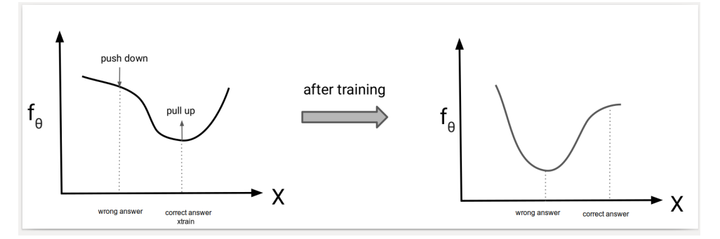
Energy-based model의 training 목표는 $\frac{\exp\{f_\theta(\mathbf{x}_{train})\}}{Z(\theta)}$의 최대화 이다. (maximum likelihood) 최대화 방향은, 식의 분자를 크게 만들고 분모를 작게 만드는 방향이다. 직관적으로 model $f_\theta$는 $\mathbf{x}_{train}$에 대해 높은 값을 가져야 한다. 그러나 $\theta$를 단순히 $f_\theta(\mathbf{x}_{train})$을 높이는 방향으로 학습하는 것이 $\mathbf{x}_{train}$이 다른 sample에 비해 상대적으로 높은 probability를 갖도록 하지는 못한다. 왜냐하면 $f_\theta$ 는 normalize 되어있지 않기 때문이다. 따라서 학습은 $\mathbf{x}_{train}$ 의 $f_\theta$ 값을 높이고 나머지 다른 sample들 ($\mathbf{x}_{sample}$)의 $f_\theta$ 값을 낮추 도록 학습 되어야 한다. 즉, wrong point에 대한 $f_\theta$의 값은 push down을 하고 correct point에 대한 $f_\theta$의 값은 pull up을 시켜야 한다.

Contrastive Divergence

앞서 말한 것처럼 partition function은 $\mathbf{x}$의 dimension이 커질 수록 연산이 어렵다. 따라서 이를 직접 evaluating 하는 것 대신 approximation하는 것이 좋다. 이때 Monte Carlo estimation을 이용할 수 있다. contrastive divergence algorithm은 Mote Carlo estimation을 이용해 gradient를 구한다.

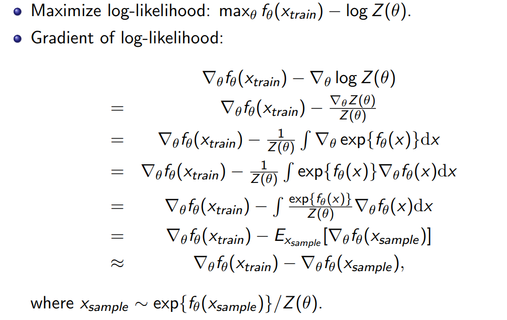
문제는 $\mathbf{x}_{sample}$을 $p_\theta$로 부터 구해야 한다는 것이다. 따라서 partiton function에 관계 없는 sampling이 필요하다.

Sampling from Energy-based Models

Energy-based model을 sampling 하는 것은 어렵다. 왜냐하면 autoregressive model이나 flow model 처럼 바로 sampling 하는 것이 어렵기 때문이다. (모델 $f_\theta$ 외에 $Z(\theta)$ 연산이 필요하다.) 그러나 enery-based model의 application에서 처럼, 두 samples를 비교하는 것은 쉽다. Markov Chain Monte Carlo(MCMC)를 이용하면 두 sample을 비교하는 방식으로 sampling이 가능하다. 아래는 MCMC 알고리즘 중 하나인 Metropolis-Hastings 을 이용한 sampling 과정이다.

1. $\mathbf{x}^0$를 random initialize.
2. $\mathbf{x}^\prime=\mathbf{x}^t + \mathrm{noise}$
   • $f_\theta(\mathbf{x}^\prime)\gt f_\theta(\mathbf{x}^t)$ 이면, $\mathbf{x^{t+1}=x^\prime}$
   • 반대의 경우 $\exp(f_\theta(\mathbf{x}^\prime)-f_\theta(\mathbf{x}^t))$의 확률로 $\mathbf{x^{t+1}=x^\prime}$
3. 수렴할 떄 까지 2번 반복

그러나 위와 같은 방식은 이론적으로 가능하지만 현실적으로 수렴하는데 너무 많은 시간이 걸린다.

Reference

cs236 Lecture 11