cs236
1.Cs236 Lecture3
Generative Model Generative model은 probability distribution을 학습한 model이다. 어떤 training dataset이 있다고 할 때, 해당 dataset을 생성하는 true unknown probability dist
2.Cs236 Lecture4

Learning A Generative Model Setting $P_{data}$: domain에 대한 underlying distribution. unknown 상태. $\mathcal{D}$: $P_{data}$로 부터 sampling한 dataset. IID:
3.Cs236 Lecture5
Latent Variable Models Motivation 사람 얼굴 이미지는 endor, eye color, hair color 등 다양한 factor들에 의해 서로 다르게 나타난다. 이러한 다양한 요인들은 이미지에 이러한 요인들이 annotation 되어 있지 않
4.Cs236 Lecture6
Intractable Posteriors 앞선 lecture에서 살펴본 대로 ELBO가 likelihood $p_{\theta}(\mathbf{x})$와 같아지는 조건은 $q(\mathbf{z})=p(\mathbf{z|x};l\theta)$일 때 뿐이다. 따라서 pos
5.Cs236 Lecture7
Simple Prior to Complex Data Distributions 직전 lecture에서 살펴본 VAE는 latent variable을 이용하여 modeling 하는 모델이다. VAE가 충분히 성공적인 모델이 될 수 있었던 이유는 simple prior($p
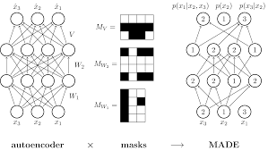
6.Cs236 Lecture8
A Flow of Transformations Normalizing flow의 normalizing은 invertible transformations을 거치면 normalized density를 얻는 다는 것을 나타내며, flow는 invertible transform
7.Cs236 Lecture9
Maximum Likelihood 방식의 학습은 빠른 학습 속도를 갖는다. 하지만 높은 likelihood가 항상 좋은 quality의 sample 생성을 보장하지는 않는다. 반대로 좋은 sample이 낮은 likelihood를 갖는 경우도 있다. (overfittin
8.Cs236 Lecture10

F-Divergence 두 개의 distribution $p, q$가 주어졌을 때 f-divergence는 다음과 같이 정의 된다. $Df(p, q)=E{\mathbf{x}\sim q}[f(\frac{p(\mathbf{x})}{q(\mathbf{x})})]$, $f$는
9.Cs236 Lecture11
Parameterizing Probaility Distribution Probaility는 다음과 같은 특징을 가진다. non-negative: $p(\mathbf{x})\ge0$ sum-to-one: $\sum_\mathbf{x}p(\mathbf{x})=1$ or $
10.Cs236 Lecture12
Sampling from EBMs: Unadjusted Langevin MCMC Unadjusted Lagevin MCMC는 다음과 같은 process를 거친다. $\mathbf{x}^0\sim\pi(\mathbf{x})$ Repeat for $t=0,1,2,\cdo
11.Cs236 Lecture13
Score-based Models 지금까지 공부한 generative models의 벤 다이어 그램을 그리면 다음과 같은 관계를 볼 수 있다. 기존 Auto-regressive model과 Flow matching model이 likelihood를 바로 최적화 하여
12.Cs236 Lecture14
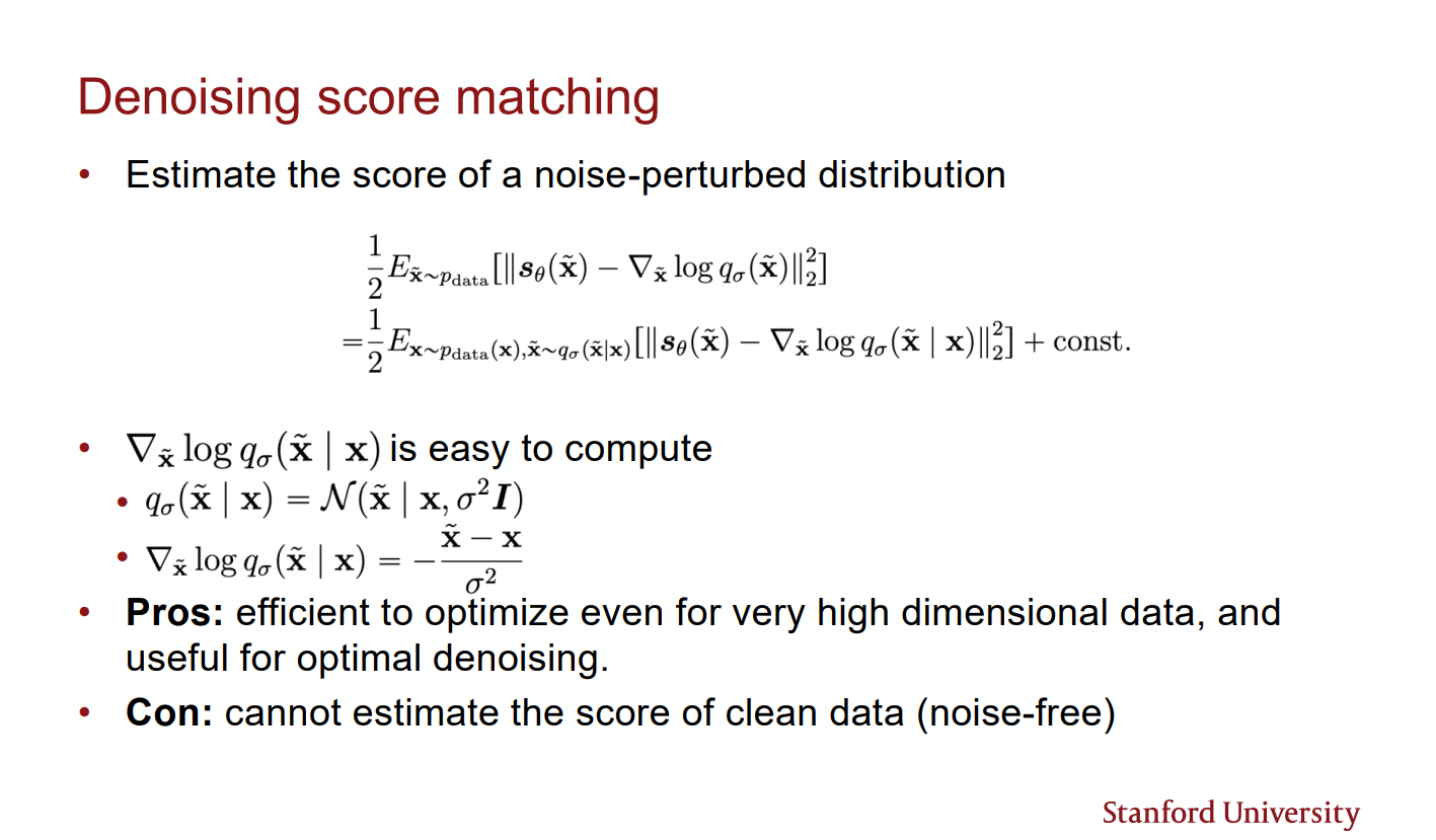
Gaussian Perturbation Score matching의 pitfalls(manfiold, low densitiy에 대한 부정확한 score estimation, 느린 mode change)는 모두 gaussian perturbation을 통해 해결 할 수
13.Cs236 Lecture15
Classifier 같은 discriminative models에 대한 evaluation은 비교적 쉽다. 왜냐하면 task-specific 한 loss를 바로 적용할 수 있기 때문이다.(e.g. top-1 accuracy) 그러나 generative models에 대
14.Cs236 Lecture16
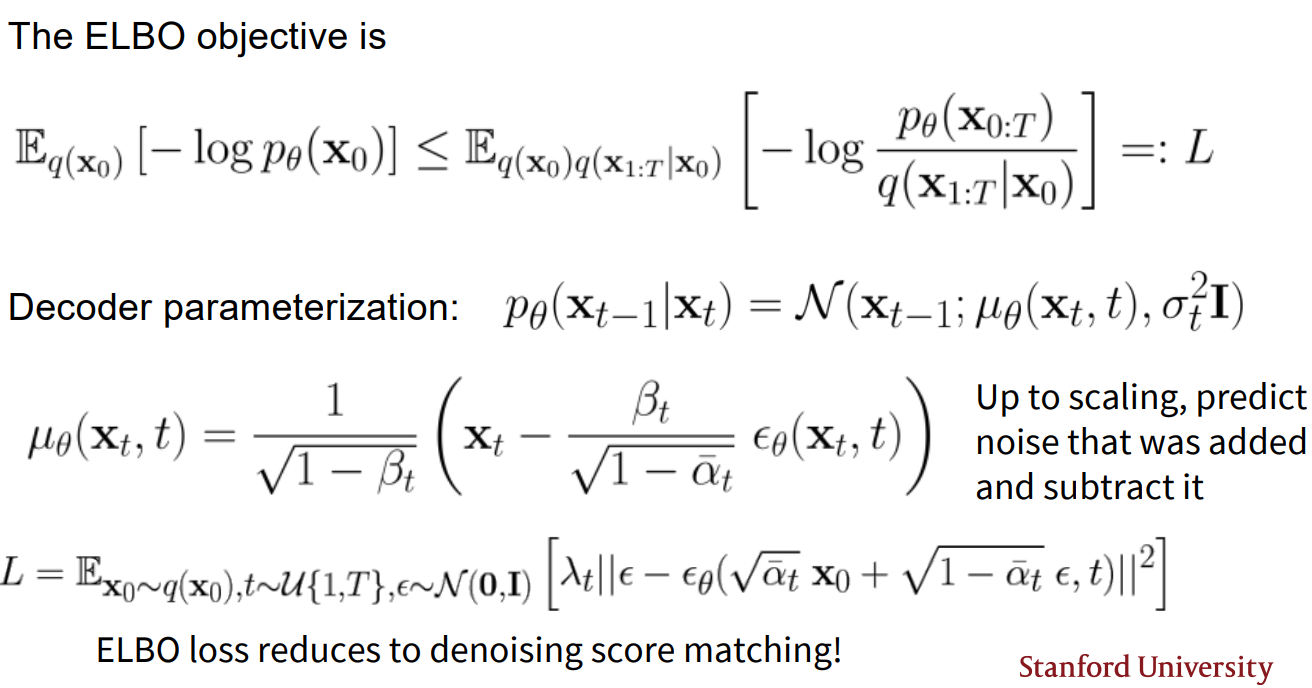
Diffusion Models Iterative Noising Process $\mathbf{x}0$ 부터 $\mathbf{x}T$ 까지 점차 noise를 더해간다. $\mathbf{x}0$는 perturbed 되지 않은 density를 가지며 $p{data}(\mat
15.Cs236 Lecture17
Converting the SDE to an ODE SDE를 Ordinary differential equation(ODE)로 변경 가능하다. ODE 식은 다음과 같다. ODE: $\frac{\mathrm{d}\mathbf{x}t}{\mathrm{d}t}=-\frac{