2.1 Distributions of two random variables (이변량분포)
Multivariate distribution 다변량 분포 중 주로 main 으로 다루는 것은 이변량이다. 그간 C에서 X(c) 로의 매핑을 다루는 단변량 확률변수를 X를 다루었다면 이제는 확률변수가 모인 확률벡터를 다루게 될 것이며, 이를 X (bold X) 로 표시한다. 명확한 정의는 다음과 같다.
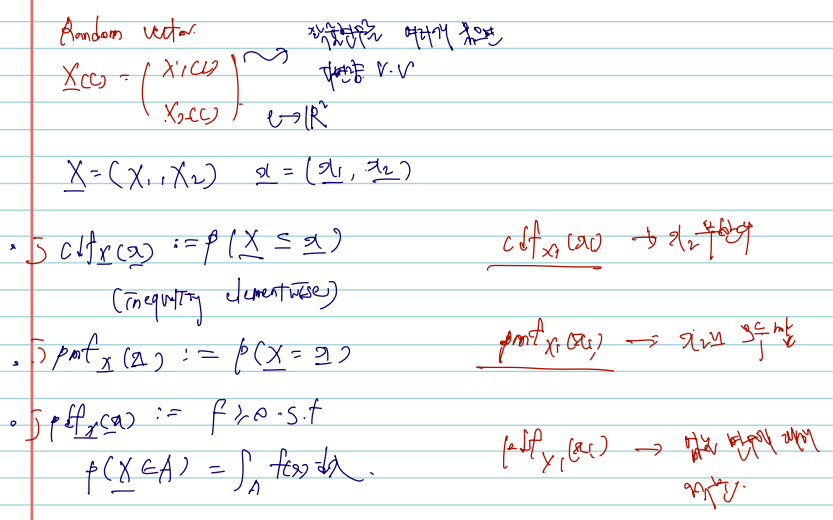
Definition X:=(X1,X2) is called a (bivariate) random vector ((이변 량) 확률벡터) if X(⋅) is a multivariate function that maps c∈C to X(c):= (X1(c),X2(c))∈R2, i.e., X:C→R2.1 An equivalent definition is that X is a random vector if each component of X is a random variable.
- 따라서 (X1(c), X2(c)) 가 모인 확률벡터가, R2에 속하여야 한다.
- vector notation 은 X=[X1X2]=(X1,X2)T 와 같이 기본으론 열벡터로 적으며 행벡터로 적고 싶다면 Transpose 형태가 된다.
- The space of X is D={(x1,x2):x1=X1(c),x2=X2(c),c∈C}.
joint cdf: 이변량 확률벡터의 cdf 는 자연스럽게 joint cdf 라 불릴 수 있으며, X2의 범위를 -무한대부터 무한대까지로 준다면 자연스럽게 FX1(x1)의 단변량을 다루는 cdf 로 전환이 가능하다.
- The joint cdf (결합누적분포함수) of X=(X1,X2)T is defined by
FX1,X2(x1,x2):=P(X1≤x1,X2≤x2)2
and can easily show
P(a1<X1≤b1,a2<X2≤b2)=FX1,X2(b1,b2)−FX1,X2(a1,b2)−FX1,X2(b1,a2)+FX1,X2(a1,a2)
- 4개의 항으로 이루어진 이 식은 X1, X2 축을 각각 그리고 square 넓이를 계산한다 생각하면 된다.
joint mgf: 이변량 확률벡터가 discrete 경우 확률질량함수는 결합확률질량함수이며, 높아진 차원에서 정의되는 확률벡터 X의 나머지 공간에서 확률이 0이면 된다. (단변량의 pmf 와 같다.) 이때 ,(comma)는, 마치 and 처럼 해석하면 된다.
- A random vector X is called discrete if there exists a countable subset S⊆R2 such that P(X∈Sc)=0. For a discrete r.v. X=(X1,X2)T, the joint pmf (결합확률질량함수) is defined by
pX1,X2(x1,x2)=P(X1=x1,X2=x2)
joint pdf: 이변량 확률벡터가 continuous 인 경우는 cdf를 통해 정의하며, 적분해서 cdf가 되는 nonnegative function 을 joint pdf 라 한다.
- A random vector X is called continuous if FX(x)=0 is continuous for every x∈R2. For the continuous r.v. X=(X1,X2)T, a nonnegative function fX1,X2(x1,x2) satisfying
FX1,X2(x1,x2)=∫−∞x2∫−∞x1fX1,X2(w1,w2)dw1dw2
is called the joint pdf (결합확률밀도함수) of X. It is easy to check that
∂x1∂x2∂2FX1,X2(x1,x2)=fX1,X2(x1,x2)
- 위 식에서 볼 수 있듯이 joint pdf 는 joint cdf 를 해당하는 각 변수에 대해 각각 편미분한 형태로 정의된다.
(more formal definition from the measure theory)
포함되는 시그마-field 를 활용한 좀 더 엄밀한 정의를 생각하면..
- Let F be a σ-field on a sample space C and B(R2) be the Borel σ-field on R2 (the σ-field generated by all open rectangles). 라 하자.
- 기존의 정의는, X:C→R 이었고 X is random variable: X−1(B)∈F. 에 속해야 했다. 이때 Borel set B∈B(R) 역시 만족.
- random vector 에서의 정의는, X가 X가 되어 radom vector 가 된다는 점, R가 높아진 dimension 에서 R2가 된다는 점 이외에 특별한 차이가 없다.
X:C→R2 is called a bivariate random vector if X is measurable, i.e., for any Borel set B∈B(R2),X−1(B)∈F.
marginal pmf, marginal pdf (주변확률질량함수, 주변확률밀도함수)
위에서 잠깐 언급했듯이, joint cdf와 joint mgf 만 주어져도 한 변수의 cdf, mgf 가 계산이 가능하며, 이는 계산하고자 하는 변수 외 다른 변수를 무한대의 범위로 확장함으로써 이루어진다. (한 변수를 고정하고 나머지 변수에 대해 적분해버리면 된다. 그렇다면 P(X1= x1)을 구하고 싶다면? X1 =x1 에 고정하고 x2에 대해 적분하면 된다.) 이에 대한 식은 다음과 같다.
- pX1(x1)=∑x2pX1,X2(x1,x2) : marginal pmf (주변확률질량함수) of X1
- fX1(x1)=∫−∞∞fX1,X2(x1,x2)dx2 : marginal pdf (주변확률밀도함수) of X1
(Example)
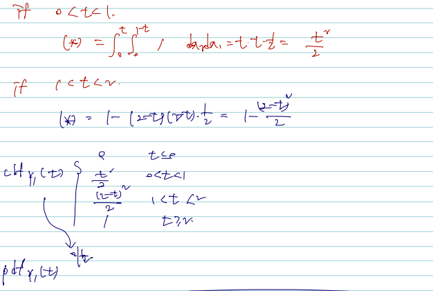
Let f(x1,x2)=x1+x2,0<x1<1,0<x2<1 be a joint pdf of X1 and X2. Compute P(X1≤1/2) and P(X1+X2≤1).
1) P(X1≤1/2) 구.
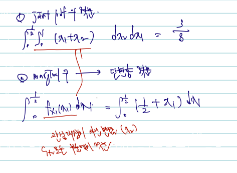
2) P(X1+X2≤1) 구.
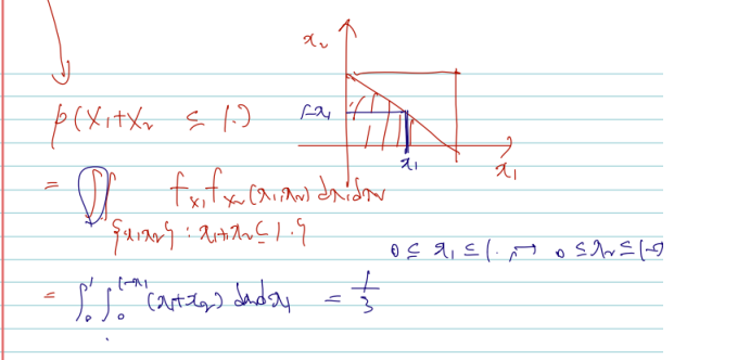
다음과 joint pdf 가 주어졌을 때 marginal cdf 를 구하는 것을 구하는 일반적인 방법은 joint pdf 를 서로 다른 두 변수에 대해 적분하거나, marginal pdf 를 구하고 단변량 적분을 하는 것이다. 그러나 여기서는 어느 방법을 택하든 결국은 marginal 을 구해서 관심 대상이 아닌 변수를 모든 부분에서 적분하여 값을 얻을 수 있음을 기억하자.
How to calculate expectations of Y=g(X1,X2) ?
다변량을 변환하는 함수 g를 입힌 Y에 대한 기댓값은, 단변량에서와 마찬가지로 g(x)f(x)를 적분해주면 된다. 단 여기서는 변수가 2개로 늘었으므로 integral & summation 을 각 변수에 대해 2번씩 해주면 된다.
E[g(X1,X2)]={∬g(x1,x2)f(x1,x2)dx1dx2∑x1∑x2g(x1,x2)p(x1,x2) if ∬∣g(x1,x2)∣f(x1,x2)dx1dx2<∞ if ∑∑∣g(x1,x2)∣p(x1,x2)<∞.
Theorem (The linearity of expectation). Let E∣g1(X1,X2)∣<∞ and E∣g2(X1,X2)∣< ∞. Then, for any k1,k2∈R,E∣k1g1(X1,X2)+k2g2(X1,X2)∣<∞ and
E[k1g1(X1,X2)+k2g2(X1,X2)]=k1E[g1(X1,X2)]+k2E[g2(X1,X2)]
다번량에서도 expectation 을 구하는 것이나 linearity of expection은 유지된다. ㅇ여기서도 전제는, 각 다변량에 대한 g1과 g2의 기댓값이 eixst 하고, 이들의 합의 기댓값도 존재해야 한다는 점. 선형 결합의 expectation 이 각자의 상수배로 연결된다.
(Example)
Let X=(X1,X2)T be a continuous random vector with joint pdf f(x1,x2)=8x1x2I(0<x1<x2<1). compute $E\left(X{1} X{2}^{2}\right).
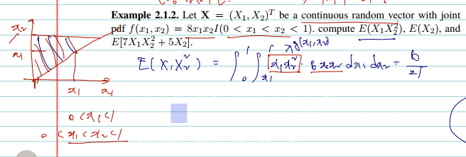
함수를 적분하는 것은 어렵지 않으나 범위에 유의하자.
Definition (joint mgf). Let X=(X1,X2)T be a random vector. The joint mgf (결합적률생성함수) of X is defined by
MX(t):=E[etTx]
변수의 m차원 적률을 생성하는 mgf도 joint 라고 변하지 않는다. 딴 X가 random vector 가 된다는 것이 차이이며, 또다른 차이로는 t가 X와 차원을 맞춰주기 위해 R2되어야 한다. 왜? 적률생성함수의 기댓값 내에서 e에 t1X1 + x2X2 이 윗첨자로 들어가기 때문이다. 따라서 t = (t1, t2)처럼 표기할 수 있다.
t는 또다시 0을 포함해야 한다.
if it is finite for all t:=(t1,t2)T satisfying ∥t∥<h for some h>0. Another expression is
MX(t)=MX1,X2(t1,t2)=E[et1X1+t2X2]
만약..joint mgf에서 margianl mgf 로 또다시 범위를 줄이고 싶다면 joint mgf가 주어졌을 때 t2 = 0 을 집어넣으면 다음과 같다. 따라서
MX1,X2(t1,0)=MX1(t1): marginal mgf of X1
(Example)
Let (X,Y) be a continuous random vector with joint pdf f(x,y)= e−yI(0<x<y<∞). Compute its joint and marginal mgfs.

joint pdf 가 주어졌을 때 margian mgf 를 구하는 것은 이전에도 그랬듯이 E 안 input 들을 모두 g(x)처럼 두면 된다. 그러면 자연스럽게 transformation 처럼 integral 2개를 사용한 적분 식으로의 전환이 가능하다. 서로 다른 두 변수에 대해 적분하므로 이 경우에도 적분 범위를 조심하자. 이 경우, 나는 자연상수 e를 포함한 적분에도 애를 먹었다.
Theorem. 이변량일 때 적률을 생성하는 mgf 의 보다 일반적인 식을 알아보자. 다음 X와 Y가 각각 a,b번 곱해진 moment 의 기댓값은 각 변수의 a, b차만큼 mgf 를 편미분 한 것과 같다.
Let M(t1,t2) be the joint mgf of (X,Y). Then, for any positive integers a and b,
E(XaYb)=∂t1a∂t2b∂a+bM(t1,t2)∣∣∣∣∣t1=t2=0
앞서서는 bivariate r.v.의 transformation expectation 을 살펴봤다면, 이제는 pdf를 구할 수 있다. joint 라고 pdf 를 구하는 것이 다르지는 않으며, 1. g(X1, X2) = Y라 할 때 Y의 cdf 를 구한 후 미분하거나 2. transformation techniques 아래를 쓴다.
(Example) Let X:=(X1,X2)T be a discret random vector with joint pmf as below. Find the pdf of Y1=X1+X2.
joint pmf 가 주어졌을 때 Transformation 의 pdf 를 구하는 문제이다. 그러나 pmf 가 joint 라면 pdf 역시 joint 로 계산되어야 하며 따라서 위 techniques 식에서 g inverse y 를 먼저 구하는 과정이 필요하다. 이때 Y1 외에도 Y2 에 대한 정의가 필요하며 one-to-one을 위해 y2= x2 로 끼워넣어주는 과정이 필요하다.
pX(x)=x1!x2!μ1x1μ2x2e−μ1−μ2,x1=0,1,2,⋯,x2=0,1,2,⋯
i.e. x1=y1−y2,x2=y2. So, the joint pdf of Y1 and Y2 is
pY1,Y2(y1,y2)∴pY1(y1)=(y1−y2)!y2!μ1y1−y2μ2y2e−μ1−μ2,(y1,y2)∈T=y2=0∑y1pY1,Y2(y1,y2)=y1!e−μ1−μ2y2=0∑y1(y1−y2)!y2!y1!μ1y1−y2μ2y2=y1!(μ1+μ2)y1e−μ1−μ2,y1=0,1,2,⋯
joint pdf 를 구했다면 marginal 위해 y2 = 0으로 고정하고 하나의 변수에 대해 계산해주면 된다.
중간정리
multivariate random vector 을 다루는 지금도 cdf, pmf, pdf 의 일반적인 관계는 옂ㅓㄴ히 유지된다. 변경된 것은 random value에서 random vector을 다루게 된 점 정도이다.
따라서 joint 가 주어질 때 그 중 하나의 변수에 대해 cdf, pmf, pdf 구하는 각각의 방법이 약간은 추가된 점이다. cdf는 구하려고 하는 변수 이외 변수를 무한대로 보내면 / pmf는 이외 변수에 대해 summation / pdf 는 이외 변수에 대해 적분해주면 되었다.
2.2.2 Continuous case
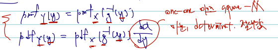
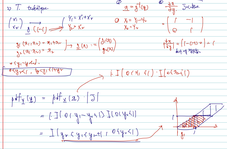
이제 확률벡터의 변환 중 연속형일 경우를 보자. (joint pdf of X를 주고 joint pdf of Y를 구하는 문제) 이 경우 확률변수에서 그랬듯이 1. f inverse(y) 역상을 구해주는 것이며 2. Jacobian 의 determinant 에 절댓값을 취해 곱해준다. 식을 보면 다음과 같다.
fY(y)=fX(w(y))∣∣∣∣∣∂y∂x∣∣∣∣∣,y∈T
where w(y)=(w1(y),w2(y))T.
단변량일 경우 이에 대한 증명이 기억나지 않아 찾아왔다. 증명에서도 보이듯, X에서 Y로 연결하는 함수 g가 one-to-one 이어야 한다.
(Jacobian의 경우도 잠깐 정리해 둔다.)
J=∣∣∣∣∣∣∂y1∂x1∂y1∂x2∂y2∂x1∂y2∂x2∣∣∣∣∣∣
(Example)
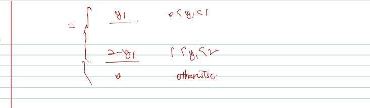
Let X=(X1,X2)T be a continuous random vector with joint pdf fX1,X2(x1,x2)=I(0<x1<1,0<x2<1). Find the pdf of Y1=X1+X2. Solve this by cdf technique and 1-1 transformation technique.
확률변수의 변환에서 흔히 사용되는 방법은 2가지로 1. cdf 를 구한 후 미분하거나 2. 1-1 transformation technique 를 쓰거나, 이다. 후자의 방법은 pdf of Y를 구하는데 있어 pdf of X를 쓴 후 바로 Jacobian 을 이용해 곱하는 방법이다. 각각 나누어 적어뒀다.
1) take cdf and derivative

2) 1-1 Transformation technique
2.3 Conditional distribution and expectation
조건부분포는 조건부 확률로부터 유도할 수 있는 conditional pmf, conditional pdf 를 말하며, joint 인 경우도 크게 다르지 않다.
Definition.
- If (X1,X2) is discrete and pX1(x1)>0, the conditoinal pmf of X2 given X1=x1 is
pX2∣X1(x2∣x1)=pX1(x1)pX1,X2(x1,x2)
- If ( X1,X2) is continuous and fX1(x1)>0, the conditoinal pdf of X2 given X1=x1 is
fX2∣X1(x2∣x1)=fX1(x1)fX1,X2(x1,x2)
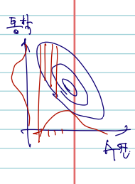
정의의 모양이 다음과 같은 이유는 직관적인 해석과도 크게 다르지 않다. X1이 수면시간, X2가 통학시간을 의미하는 다음과 같은 분포가 있다고 하자. 다음과 같은 contour
plot 은 높이가 같은 선들을 이은 것이며, 여기서는 해당하는 사람들의 수가 될 것이다. 조건부 확률은, 여기서 예컨대 X1 = x1 수면시간을 6시간으로 고정해두고, 그때 6시간 자는 사람들의 X2 통학시간의 분포를 궁금해하는 것이 된다. 그럼 분모는 사실상 x1으로 고정해두고 pdf 를 X2에 대해 적분한 값의 역수가 된다. 이 역숫값 c가 아래 continous case 의 분모라 생각하면 쉽다.
조건부분포의 pmf, pdf 말고 기댓값을 구할 수 있는데, 이 역시 X1= x2 은 고정해둔 채 X2의 기댓값을 구하는 것이다.
Conditional expectation (조건부 기댓값) of u(X2) given X1=x1 :
E[u(X2)∣x1]4=∫−∞∞u(x2)f(x2∣x1)dx2
조건부 분산은 다음과 같다.
Conditional variance of X2 given X1=x1 :
Var(X2∣x1)=E[{X2−E(X2∣x1)}2∣x1]=E(X22∣x1)−E2(X2∣x1)
분산에 대해 조건부일 경우와 그렇지 않은 경우를 비교하면 다음과 같다.
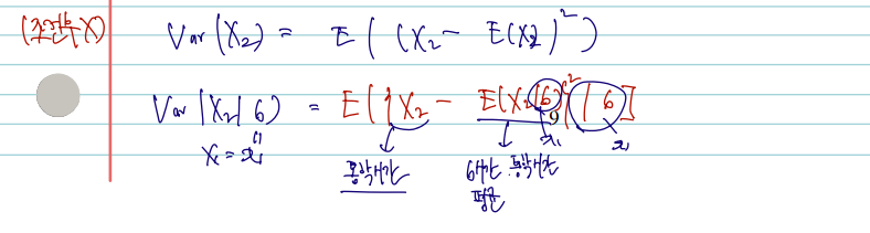
6시간 자는 사람들 중 통학시간 분포의 분산을 구하려고 하면, 1. 통학시간에서 2. 수면시간 6시간인 사람들의 통학시간 평균 을 빼면 될 것이고, 이를 x1=6일 때에서 찾으면 될 것이다.
(Example)
Find EX1∣X2(X1∣x2) and VarX1∣X2(X1∣x2) when f(x1,x2)= 2I(0<x1<x2<1).
joint pdf 가 주어졌을 때 이들의 cond'l Expectation, Variance 를 구하는 문제이다. 우선 조건부 분포의 pdf를 잘 알아야 하겠고.. 이를 위해 pdf of x2를 구해야 하는 번거러운 계산도 필요하다. 그러나 이 과정을 넘기면 적분 범위만 조심하며 '산수'를 하면 된다.

Theorem (Double expectation theorem)*
Double expectation theorem은 조건부 기댓값에 기댓값 또는 분산을 씌웠을 때에 관한 것이며 전 확률의 정리(the law of total probability)의 일반화이다. 특히 a와 관련해서는 우변에서 좌항으로의 변화를 잘 기억해두면 요긴하게 쓰일 수 있다.
(a) E[E(X2∣X1)]=E(X2).
(b) Var(E(X2∣X1))≤Var(X2)=Var[E(X2∣X1)]+E(Var(X2∣X1)).
(pf)
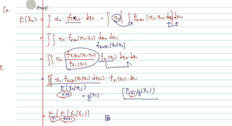
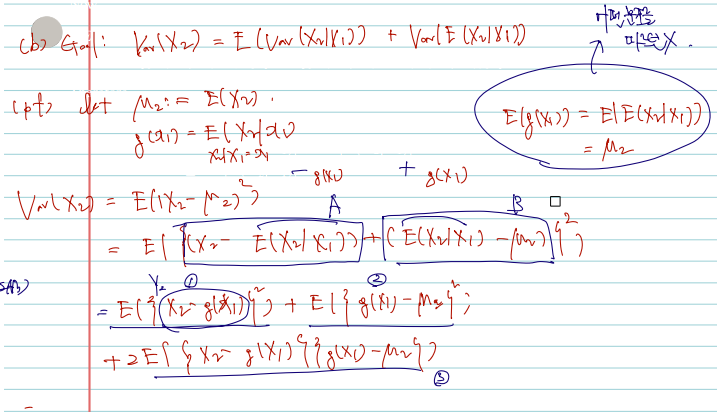
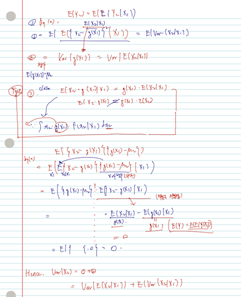
증명의 호흡이 길 순 있으나, 조건부 기댓값/분산의 정의, 어떤 변수에 대한 적분인지, 적분의 선형성 등만 익히고 있다면 아주 재미나게 증명할 수 있다. 아, 또한 given X1=x1일 때 X2의 expectation 은 g(x1) 함수로 볼 수 있다는 사실도 기억해두자.
