[Mathematical Statistics] 6.3 Likelihood ratio test

Review

6.2절은 내용이 중요하면서도 다른 이전 절의 fact 까지도 끌어와서 사용하기에 statement 자체와 증명 과정을 음미할 필요가 있다. 이번 포스팅에도 반복되는 내용이 있기 때문에, 잠깐 리뷰하도록 하자.

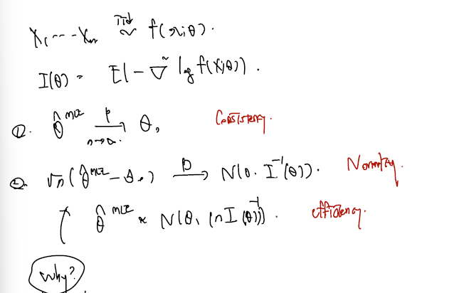
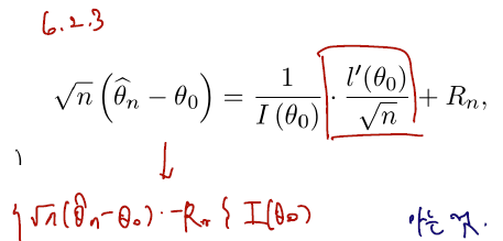
6.2절의 결론은 모수를 추정하는 unbiased estimator MLE 세타가 위와 같은 성질들을 가지고 있기에 'MLE가 다른 어떤 추정량에 뒤지지 않는다!' 라고 말할 수 있었다. 그 근거로.. 1. MLE 세타가 n이 무한대로 감에 따라 true parameter로 in prob. 수렴한다는 consistency 2. MLE 에서 적절히 true parameter 를 빼주고 n의 square root 를 곱한 통계량이 normal 로 in distribution 수렴한다는 normality. 3. 이때 normal 에서의 분산이 Rao-Cramer 하한인 Fisher information $nI(\theta)^-1$ 를 asymptotically follows 한다는 efficiency 가 중요했다. 이 세가지가 바로 추정량 MLE 를 특별하게 만드는 성질들이었으며, 특히 efficiency 의 경우 우리가 알고 있는 모평균의 추정량 표본평균 등은 점근적 상황을 도입하지 않고도 바로 R-C lower bound 를 touch 한다는 것을 보였다.

그리고 noramlity 보이기 위해서.. 세타에 대한 likelihood estimation 한 번 미분한 것을 true parameter 를 가지고 근사하는 테일러 전개를 했다.

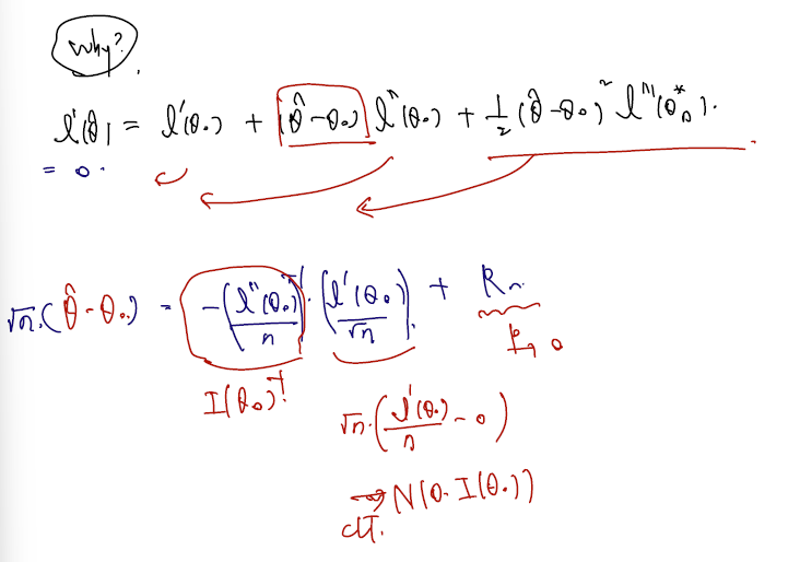
MLE 정의에 따라 log-likelihood 한 번 미분한 것에 MLE 값을 집어넣으면 0이므로 이 식은 = 0 으로 정리할 수 있고, 따라서 (MLE - true para) 이 부분만 남기고 정리하면 다음과 같다.

• 정리 후에 양변에 square root n 을 곱해준다.
• 두 번 미분한 것엔 / n 해주고
• 한 번 미분한 것엔 / square root n 해주면 딱 들어맞고..
• 각각 inverse Fisher information (by WLLN), $N(0, I(\theta_0))$ (by CLT), op(1) 이라는 것을 증명했다. (remained term 증명이 오히려 가장 까다로웠다. 핵심에 집중하는 게 나을 듯)
• 그러면 inverse Fisher information 을 끼워넣을 수 있다.

결과적으로 $N(0, I(\theta_0)^-1)$ (by Slutsky's theorem) 임을 증명할 수 있었다.

6.3 Likelihood ratio test (가능도비 검정)

[1] Likelihood ratio test (LRT)

가능도비 검정의 내용을 보자. 가능도 비 검정 역시 이전 절에서 다룬 검정에 포함되는 내용이며 test statistic / null distribution / 기각역을 한 단계씩 세우는 과정을 거친다. 어떤 부분에서 특별한지 보자.

Let $X_{1}, \cdots X_{n}$ be r.s. from pdf $f(x ; \theta), \theta \in \Omega \subset \mathbb{R}$. For a point null hypothesis

귀무가설은 unknown theta 가 세타0 (e.g. 0또는 1 등등..) 과 같다고 세우고, 대립가설은 같지 않다는 양측검정이라 할 때, test statistics 은 다음과 같다.

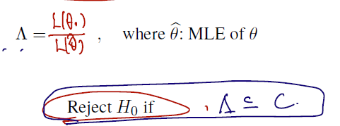
• 람다로 대부분 표기하는 LRT 통계량은 '비'로 정의되며
• 분모는 Likelihood function 에 MLE 추정량세타가,
• 분자에는 Likelihood function 에 세타 0 (known 으로 고정된 점) 이 들어간다.
• MLE 의 정의에 따라, 분모는 1일 것이고..
• 세타0를 집어넣으면 1보다 작은 가능도함수 값이 튀어나올 것이다.
• 이 값이 차이가 많이 날 경우 람다값은 더 작아지게 되고, 많이 작아질 때 (기각역 C보다 작아질 때) 귀무가설을 기각한다.

Such a test procedure is called likelihood ratio test (LRT; 가능도비검정).

Example 6.3.1 (Exponential distribution). Let $X_{1}, \cdots X_{n}$ be r.s. from $f(x ; \theta)=$ $\frac{1}{\theta} e^{-x / \theta}$, i.e. $\Gamma(1, \theta)$ or $\operatorname{Exp}(\theta)$. Derive the LRT of level $\alpha$ for testing $H_{0}: \theta=\theta_{0}$ against $H_{1}: \theta \neq \theta_{0}$.
(sol)

• exponential 함수에서의 유의수준 알파에서 귀무가설을 기각할 지 말지 결정하는 test 를 만들어보면 다음과 같다.

1) LRT 통계량 쓰기 위해 MLE 를 먼저 구하고, Likelihood 에 집어넣어 비 구하기.

2) t로 치환. g(t) <= C 가 되는 양측을 각각 C1, C2 라 하고 null distribution 구하기

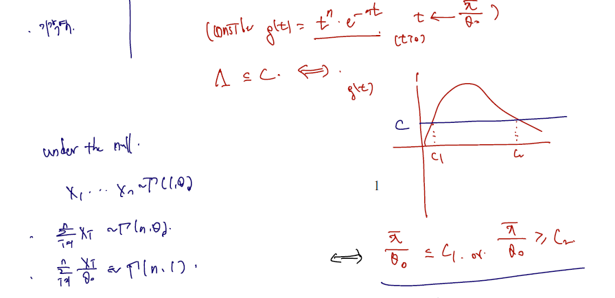
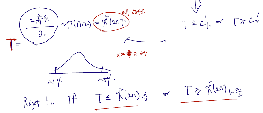
카이제곱(2n) 의 quantile of $\alpha/2$, $1-\alpha/2$ 에서 기각역이 만들어질 것이다.

Example (The mean of normal distribution with known variance). Let $X_{1}, \cdots, X_{n}$ be r.s. from $N\left(\theta, \sigma_{0}^{2}\right)$ where $\sigma_{0}^{2}$ is known. Derive the LRT of level $\alpha$ for testing $H_{0}: \theta=\theta_{0}$ versus $H_{1}: \theta \neq \theta_{0}$.
(sol)

• $L(\theta)=\left(2 \pi \sigma^{2}\right)^{-n / 2} \exp \left[-\sum\left(X_{i}-\theta\right)^{2} / 2 \sigma_{0}^{2}\right]$
• Derive $\widehat{\theta}^{\mathrm{MLE}}=\bar{X}$ (exercise!).
• So $\Lambda=L\left(\theta_{0}\right) / L(\widehat{\theta})=\exp \left[-n\left(\bar{X}-\theta_{0}\right)^{2} / 2 \sigma_{0}^{2}\right]$.
• Note that $\Lambda \leq c$ is equivalent to $\left(\frac{\bar{X}-\theta_{0}}{\sigma / \sqrt{n}}\right)^{2} \geq c^{\prime}$ for a constant $c^{\prime}$.
• Under the null, $\left(\frac{\bar{X}-\theta_{0}}{\sigma / \sqrt{n}}\right)^{2} \sim \chi^{2}(1)$
  $\therefore$ Reject $H_{0}$ if and only if $\left(\frac{\bar{X}-\theta_{0}}{\sigma / \sqrt{n}}\right)^{2} \geq \chi_{\alpha}^{2}(1)$

[2] Asymptotic null distribution of the LRT statiscits

다음에 이어질 내용은 LRT 가 어느 상황에서도 따를 수 있는 점근분포의 유도에 대한 내용이다. 결론부터 이야기하면, LRT 통계량 람다에 -2log 를 살짝 끼워넣은 것은 점근적으로 카이제곱(1)을 따르며, 이것이 null distribution 이 된다.

Theorem Assume R0-R5 are satisfied. Then, under $H_{0}: \theta=\theta_{0}$,

증명을 위해 다음 corollary 를 쓴다.

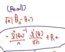
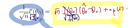
Corollary

where $R_{n}=o_{p}(1)$.

이는 위에서 금방 리뷰한 내용 중 MLE 추정량의 normality 유도 때 썼던 식이다. (편의를 위해 두 번 미분한 것은 분모에 n, 한 번 미분한 것은 루트 n, 나머지 remained term이라 생각하자.)

그러면 위 theorem 을 이제 증명할 수 있다. 출발은, MLE 추정량을 근사하기 위해 세타0에서 시작하여 테일러 전개를 하는 것이다.

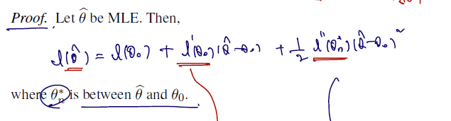
(두 번 미분 term)

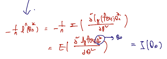
• Because $\widehat{\theta} \xrightarrow{P} \theta_{0}$ we have $\theta_{n}^{*} \xrightarrow{P} \theta_{0}$, and therefore, $-\frac{1}{n} l^{\prime \prime}\left(\theta_{n}^{*}\right) \xrightarrow{P} I\left(\theta_{0}\right)$.

(한 번 미분 term)

• 파란색 필기를 뺴고 보자.
  

따라서 위 두 term 을 이용하여 처음부터 전개하면 다음과 같다.

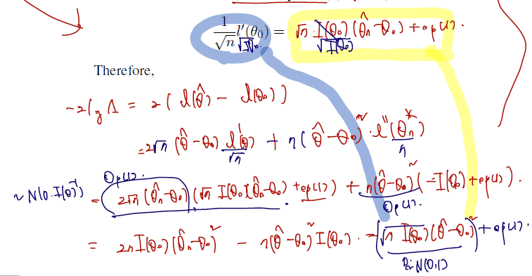
마지막 결과가 N(0,1) 을 따른다는 것은 다음을 쓰면 된다.

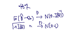
따라서 N(0,1)^2 + op(1) 이 점근적으로 따르는 (convergence in distribution) 분포는 카이제곱(1) 이다.

[3] Wald and score tests

• Wald-type test statistic:
  $\chi_{W}^{2}:=\left\{\sqrt{n I(\widehat{\theta})}\left(\widehat{\theta}-\theta_{0}\right)\right\}^{2} \xrightarrow{D} \chi^{2}(1)(\text { why? })$

Wald-type test statistics 는 갑자기 떨어진 것이 아니라, 바로 위 $-2 \log \Lambda$ 가 따르는 증명을 할 때 마지막 항에서 remained term 을 빼고 쓴 것이다. 이때 모르는 통계량 대신 MLE 추정량이 true parameter 로 in probability converge 하는 것을 이용해 MLE 로 바꿔서 쓴다. 따라서 다음과 같다.

Note that $-2 \log \Lambda=\chi_{W}^{2}+o_{p}(1)$, i.e., the LRT statistic and $\chi_{W}^{2}$ are asymptotically equivalent. -> n커지면 op(1) 은 0으로 간다는 뜻이므로.. 점근적으로 카이제곱(1)로 수렴한다는 점에서 같다.

• Rao's score test statistic:
  $\chi_{R}^{2}:=\left\{l^{\prime}\left(\theta_{0}\right) / \sqrt{n I\left(\theta_{0}\right)}\right\}^{2} \xrightarrow{D} \chi^{2}(1) \text { (why?) }$

From (1), one can also derive $\chi_{s}^{2}=\chi_{W}^{2}+o_{p}(1)$, i.e, two test statistics are asymptotically equivalent.

라오 통계량도 갑자기 떨어진 것이 아니고.. Wald-type 통계량 대신 root 를 씌운 것을 교체해서 쓴 것 뿐이다.

(각 변을 $I(\theta_0)$ 으로 나누고 좌변의 식 이용한 것이 Rao score)

From (1), one can also derive $\chi_{s}^{2}=\chi_{W}^{2}+o_{p}(1)$, i.e, two test statistics are asymptotically equivalent.

정리하면 LRT, Wald, score 통계량은 표현만 다르지 셋 모두 카이제곱(1)로 점근적으로 수렴한다는 점에서 공통된다. 따라서 test 성격에 따라, 검정력에 따라, 실험에 따라 셋 다를 쓸 수도, 그 중 원하는 통계량을 골라 test 할 수도 있겠다.