[Mathematical Statistics] 6.2 Rao-Cramer lower bound and efficiency

6.2 Rao-Cramer lower bound and efficiency

라오 크래머 하한은 본 확률 통계학 전체 내용 중 가장 중요한 내용이자 이전에 다룬 많은 사실관계들이 동원되는 내용이다. 호흡도 길고 하니.. 본 포스트의 내용을 잘 정리해두면 좋겠다.

먼저 라오-크래머 하한을 통해 보여주고 싶은 목표를 보자.

Goals

• 1. To establish a lower bound (Rao ${ }^{1}$-Cramér lower bound, 라오 크래머 하한) on the variance of any unbiased estimator.
• 2. To show that MLE asymptotically follows the normal distribution.
• 3. To show that (under regularity conditions) the asymptotic variance of MLE achieve the RaoCramér lower bound.

1. 은 라오-크래머 하한을 증명하고 자유롭게 쓸 수 있게 된다면.. 어떤 unbiased estimator 에 대해서도 lower bound 를 쓸 수 있게 됨을 뜻한다. 그리고 나서 3으로 넘어가기 위해 우리는 2. MLE 가 항상 normal distribution 을 asymptotically 따른다는 것을 보일 것이고.. 이를 통해 3. MLE 의 asymptotic variance (n이 무한대로 갈 때 variance)는 항상 R-C bound 를 touch 함을 보일 것이다.

결론적으로 MLE 는 다른 증명 없이도 nice 한 추정량임을 보이기 위한 내용들이다. 그러나 1, 2, 3, 특히나 본격적으로 R-C lower bound 를 보이기 위해선 다음과 같은 내용을 하나씩 봐야 한다.

• 1. Bartlett identity
• 2. Score function and Fisher information

[1] Bartlett identity

Bertlett identity 를 보이기 위해선 확률변수 X가 pdf of $f(x;\theta)$ 로부터 나왔을 때 이들의 적분구간에서 적분이 1이라는 것에서 출발한다.

We begin with the identity

$\theta$ 에 대해 미분하면 값이 0인 다음 식을 얻을 수 있다.

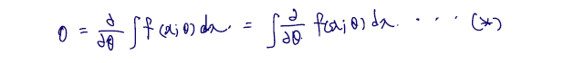
이 식의 값을 변형하지 않고 분모분자에 pdf of X를 다시 넣으면 다음과 같은 식을 얻는다. 이 식을 (1) 이라 하자.

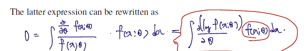
expectation 은 각 확률변수 Xi과 각 확률변수가 관찰될 확률값 (pdf of X) 을 summation 한 것이므로.. 다음 아래와 같이 쓸 수 있고, 이를 first Bartlett identity 라 한다.

(first Bartlett identity에 굳이 해석을 덧붙이면 pdf 에 log 를 취한 것을 세타에 대해 한 번 미분한, 것의 기댓값은 0이라는 것이다.)

이제 1이라 했던 식을 곱의 미분법으로 한 번 더 미분하게 되면 다음과 같은 결과를 얻는다.

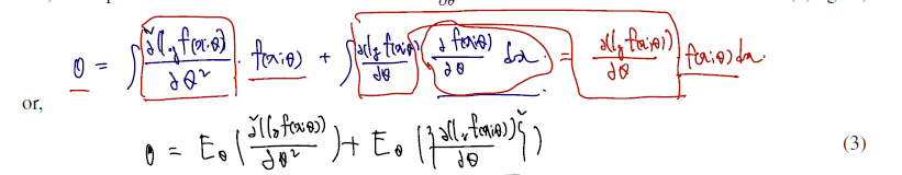
뒤 로그함수의 미분을 제곱한 것에 expectation 을 취한 것을 조금 뜯어보면.. 다음과 같이 쓸 수 있다.

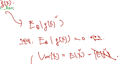
first identity 에 따라 한 번 미분한 것 (=: g(x)) 의 expectation = 0이므로 E(g(x)^2) = Var(g(x)) 라고 할 수 있다. (Var(g(x))에서 E(g(x))^2 = 0이므로)

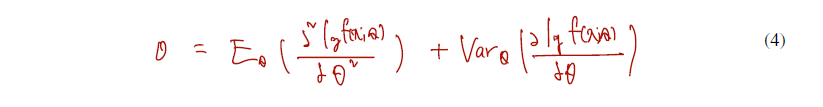
따라서 E(두 번 미분) + E(한 번 미분의 제곱) 위 식을 second Bartlett identity 라 하자.

[2] Score function and Fisher information

스코어 함수와 피셔 정보는 이의 성분을 다시 쓴 것에 지나지 않으므로 바로 살펴볼 수 있다. 정의를 살펴보자.

Definition. Let $X$ follows pdf $f(x ; \theta), \theta \in \Omega$, where $\Omega \subset \mathbb{R}$ is an open interval. (i.e., the model family is $\{f(\cdot ; \theta): \theta \in \Omega\})$ Then,

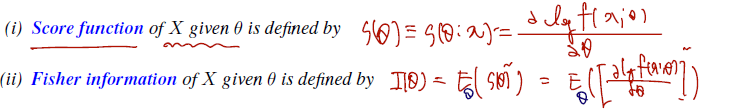
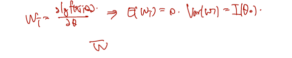
• 스코어 function 은 first identity 에 들어갔던 확률변수 같은 것을 세타에 depend 하는 함수로 빼온 것이다. log pdf (나중엔 log likelihood 로 봐야한다.) 에 한 번 미분한 것이 score function 이다.
• 피셔 information 은 score function 의 제곱의 expectation, 즉 second Bartlett identity 에 두 번째 term 과 같다.

따라서 다음과 같이 쓸 수 있다.

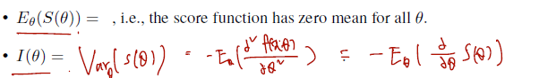
• Score function 의 기댓값은 = 0
• fisher information 은 variance of score function 으로 쓸 수 있으며, second identity 에서 이항하면 두 번 미분한 것의 expectation 에 - 를 붙인 것이다.

그렇다면 아래 예제를 통해 first Bartlett identity 가 실제로 그러한지, 로그 pdf 의 expectation 이 실제로 0인지 확인해보면 다음과 같다.

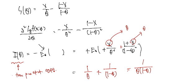
Example (Information of Bernoulli Random Variable). Let $X \sim B(1, \theta)$. Find the information of $B(1, \theta)$.
(sol)

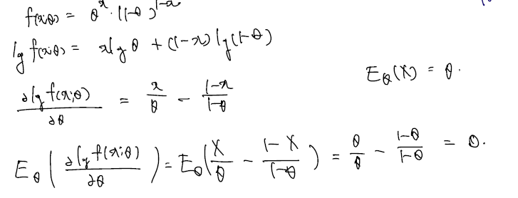
베르누이의 expectation 이 세타임을 알고 쓰면, 바로 score function expectation = 0 (Bartlett identity 1) 을 증명할 수 있다.

아래는 그렇다면 Bernouli Random Variable 의 Fisher Information 은 어떻게 쓸까 하는 것이다. Fisher Information 은 한 번 미분 제곱의 expectation, 또는 그냥 variance, 또는 두 번 미분 expectation 의 minus 각각의 표현이 있으므로 여기서 골라쓰면 된다.

Example (Information of random sample). Let $X_{1}, X_{2}$ be r.s. from $X$ following pdf $f(x ; \theta)$. Let $I(\theta)$ is the information of $X$ given $\theta$ then the information for $X_{1}$ and $X_{2}$ given $\theta$ is$=2 I(\theta)$.

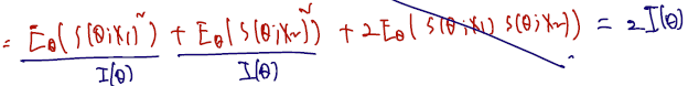
• 사실 Score function 이나 Fisher information 이나 pdf에서 one sample를 가지고 계산하는 것인데, 만약 이를 pdf 에 대해 iid 로 X1, X2 2개로 추출했다고 하자.
• 그때의 score function 은 다음과 같고 (iid Sample 에서 X1, X2 관찰할 Score 값은 각각 관찰할 Score 값의 합과 같다.)
  
• 둘을 포괄하는 information 을 그냥 $I(\theta)$ 로 쓰면 cross product 가 0이 되어 1 sample information 의 2배로 쓸 수 있다.
  
  

이를 확장하면, 확률변수 X1 ,...., Xn을 샘플링한 상황이라면 이들의 information 은 In general, the information for $n$ r.s. $X_{1}, \cdots, X_{n}$ is $n I(\theta)$.

[3] Rao-Cramér lower bound.

Theorem Let $X_{1}, \ldots, X_{n}$ be iid with common pdf $f(x ; \theta)$ for $\theta \in \Omega$. Assume that the regularity conditions $(R 0)-(R 4)$ hold. Let $Y=u\left(X_{1}, X_{2}, \ldots, X_{n}\right)$ be a statistic with mean $E_{\theta}(Y)=$ $E_{\theta}\left[u\left(X_{1}, X_{2}, \ldots, X_{n}\right)\right]=: k(\theta)$. Then

• Y는 X1...Xn 까지를 통해 만들어낸 통계량이라 하자.
• 이들의 expectation 을 $k(\theta)$ 로 두면,
• 통계량 Y의 variance는 다음과 같은 lower bound 를 가진다.
• 여기서 갑자기 튀어나오는 것이 이전에 봤던 n개 Random sample 의 fisher information 이고.. 이것이 분모로 가고, expectation 의 미분은 분자로 간다.

여기서 만약 expectation of Y 를 세타라고 한다면 (estimator 의 expectation 이 세타라는 건 estimator 가 unbiased estimator 라는 조건이었다; 비편향추정량), 이를 미분한 $k'(\theta)$ 는 1이므로 다음과 같이 쓸 수 있다.

i.e., the variance of any unbiased estimator is lower bounded by the inverse of the Fisher information. 즉, 임의의 비편향추정량의 variance 는 Fisher information 의 역수를 lower bound 로 가진다.)

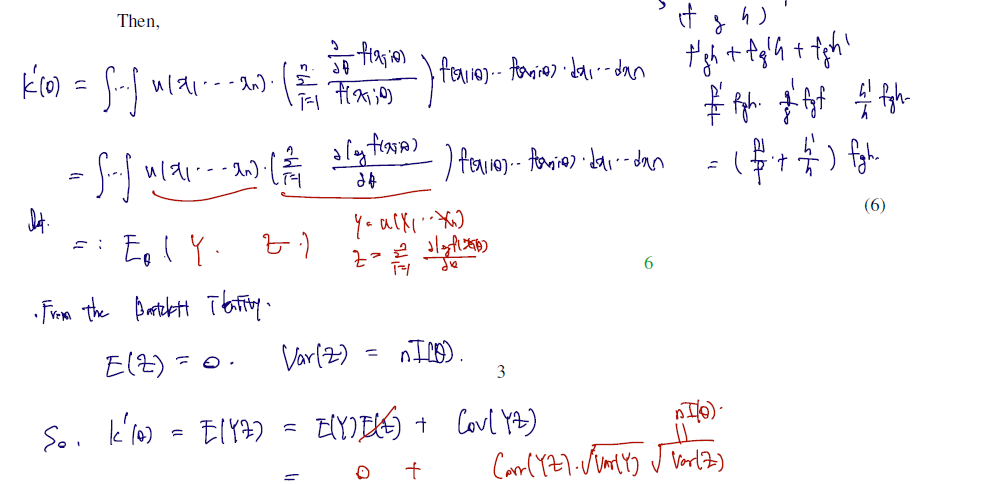
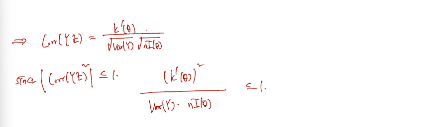
(Proof for Theorem) The proof is for the continuous case, but the proof for the discrete case is quite similar. Write the mean of $Y$ as

Then,

[4] Efficiency

효율성, 효율비의 정의를 보자. 효율추정량이란 그 추정량의 variance 가 R-C lower bound 와 정확히 일치하는 경우를 말한다.

Definition (Efficient Estimator). Let $Y=u\left(X_{1}, \ldots, X_{n}\right)$ be an unbiased estimator of a parameter $\theta$ given a random sample with size $n$. The statistic $Y$ is called an efficient estimator(효율추정량) of $\theta$ if and only if $\operatorname{Var}(Y)=1 /\{n I(\theta)\}$.

그렇지만 (뒤에서 다룰 MLE의 경우를 제외하고) 다른 추정량들은 lower bound 와 일치하거나 asymptotically 라도 일치하지 않는 경우가 많기에, 다음과 같은 비를 계산하게 된다.

Definition (Efficiency). Let $Y=u\left(X_{1}, \ldots, X_{n}\right)$ be an unbiased estimator of a parameter $\theta$ a random sample with size $n$. Then, the the efficiency (효율비) of $Y$ is defined by

만약 이 효율비가 1이라면 그 추정량은 이미 그 자체로 효율추정량이다. 만약 1보다 작다면 Var(Y)가 컸다는 이야기이므로 1보다 작은만큼 효율적이지 못하다고 할 수 있다.

실제로 X1..,Xn 을 포아송 분포에서 추출했다고 했을 때, 샘플로부터 얻은 MLE 추정량의 variance과 fisher information 역수를 비교해 비가 어떻게 되는지, (혹은 일치하는지 살펴보자.)

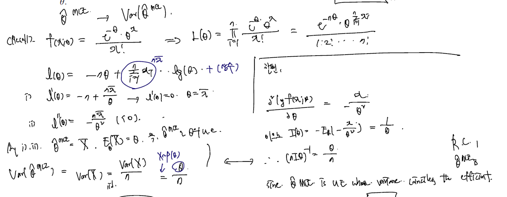
• 샘플로부터 얻은 MLE 추정량은 $\theta/n$ 이다.
• 두 번 미분한 것의 minus expectation 인 fisher information 은 $1/\theta$
• 여기에 n을 곱해줘야 하므로 일치.
• MLE 추정량은 세타의 unbiased estimator 이면서 (그래야 미분이 1이므로 식이 된다.) variance 가 Rao-Crammer 하한을 터치하므로 efficient 하다라 말할 수 있다.

[5] Asymptotic normality
그런데 우리는 추정량의 variance 가 fisher information 의 역수와 '완전히' 일치하는 경우만큼 n이 무한대로 갈 상황에서 efficienty를 고려해야 한다. 이를 위해 우선, MLE가 normality 를 따른다는 것을 보여야 한다. 다음의 R5 가정은 이를 보이기 위해 세 번 미분이 가능하고 이것이 세타에 의존하지 않는 변수의 함수로 upper bound 됨을 추가한다.

(R5) The pdf $f(x ; \theta)$ is three times differentiable as a function of $\theta$. Further, for all $\theta \in \Omega$, there exist a constant $c$ and a function $M(x)$ such that

with $E_{\theta_{0}}[M(X)]<\infty$, for all $\theta_{0}-c<\theta<\theta_{0}+c$ and all $x$ in the support of $X$.

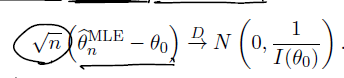
그러면 다음 정리를 쓸 수 있다. MLE 는 n이 무한대로 가면 normal로 수렴하되 분산은 fisher information 의 역수다.

Theorem Assume $X_{1}, \ldots, X_{n}$ are iid with pdf $f\left(x ; \theta_{0}\right)$ for $\theta_{0} \in \Omega$ such that the regularity conditions R0-R5 are satisfied. Suppose that the Fisher information satisfies $0<I\left(\theta_{0}\right)<\infty$. Assume further that $\left\{\widehat{\theta}_{n}^{\mathrm{MLE}}\right\}_{n}$ be a sequence of MLEs such that $\widehat{\theta}_{n}^{\mathrm{MLE}} \xrightarrow{P} \theta_{0}{ }^{2}$. Then,

이를 다음과 같이 쓸 수 있다. (asymptotically follows)

Proof. Let $\widehat{\theta}_{n}=\widehat{\theta}_{n}^{\mathrm{MLE}}$. The 1st-order Taylor expansion of $l^{\prime}(\theta)$ about $\theta_{0}$ and $\theta \leftarrow \widehat{\theta}_{n}$ gives

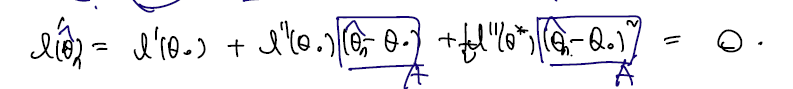
true 세타를 세타0, MLE 세타를 MLE hat 이라 할 때, 위 테일러 전개를 쓸 수 있고..이 식이 0이므로 다음을 쓸 수 있다.

(1) 차이로 묶고,

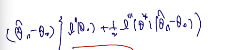
(2) 차이에 대해 정리한 다음 루트 n 곱, n으로 나누자.

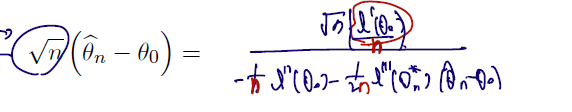
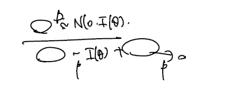
이제 각각 분모는 $N(0, I(\theta_0))$ 로, 분포는 $I(\theta_0)$ 와 0으로 수렴함을 보이면 끝난다.

(1) CLT에 의해 분자는 $N(0, I(\theta_0))$ 로 수렴

(2) WLLN 로 분모 첫항은 $I(\theta_0)$ 으로 수렴.

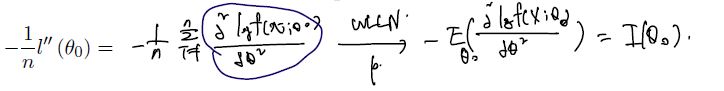
(3) 마지막 항은 0으로 in probability 수렴하는 것에 대해 bound 되어 0으로 수렴. (R5 조건의 도움을 받는다.)

따라서 분자는 Normal, 분모는 I(theta) 로 in prob. 0으로 in prob. 수렴하므로 슬러츠키 정리에 의해 이를 끼워넣을 수 있다. 따라서 다음 이어지는 내용을 위해, MLE 는 asymptotically 분산이 inverse fisher information 인 normal 을 따름을 기억하자.

[6] Asymptotic efficiency

앞선 내용들에 기반해, 보여주고 싶은 건 MLE 는 결국 n이 무한대로 가면 어떤 상황에서건 R-C lower bound 를 touch 한다는 것이다. 아래를 보자.

Definition Let $X_{1}, \ldots, X_{n}$ be independent and identically distributed with probability density function $f(x ; \theta)$. Suppose $\hat{\theta}_{1 n}=\hat{\theta}_{1 n}\left(X_{1}, \ldots, X_{n}\right)$ is an estimator of $\theta_{0}$ such that $\sqrt{n}\left(\hat{\theta}_{1 n}-\theta_{0}\right) \xrightarrow{D}$ $N\left(0, \sigma_{\hat{\theta}_{1 n}}^{2}\right)$. Then

• 만약 추정량이 $N(0, \sigma^2/n)$ 을 점근적으로 따른다는 가정을 길게 쓴 것이고, 이럴 경우

(i) The asymptotic efficiency (점근효율비) of $\hat{\theta}_{1 n}$ is defined to be

추정량의 효율비도 다음과 같이 쓸 수 있다. 여기선 점근적으로 따른다는 가정이 있으므로 똑같이 점근효율비라 쓰고, 이 비율이 1이 될 때 (n이 무한대로 갈 때 R.C lowr bound 와 추정량 자체가 점근적으로 따르는 분산이 같을 때) 이를 점근효율적 추정량이라 한다.

(ii) The estimator $\hat{\theta}_{1 n}$ is said to be asymptotically efficient (점근효율적) if the ratio in part (a) is 1 .

만약 추정량이 2개라면 어떨까? 서로 다른 추정량 중 무엇이 좋을 지 비교하기 위해선 이들의 variance 만 비교하면 될 것이다.

(iii) Let $\hat{\theta}_{2 n}$ be another estimator such that $\sqrt{n}\left(\hat{\theta}_{2 n}-\theta_{0}\right) \xrightarrow{D} N\left(0, \sigma_{\hat{\theta}_{2 n}}^{2}\right)$. Then the asymptotic relative efficiency (ARE, 점근상대효율비) of $\hat{\theta}_{1 n}$ to $\hat{\theta}_{2 n}$ is the reciprocal of the ratio of their respective asymptotic variances; i.e.,

• 만약 1보다 크다면 추정량 1이 효율
• 만약 2보다 작다면 추정량 2가 효율적이다, 라고 할 수 있다.

가장 중요한 것은 MLE 는 asymptotically eifficient estimators 라는 점이다. 위 점근효율비 정의에서, 이를 MLE 로 갈아끼우게 되면 MLE 분산이 그대로 Fisher informaiton 과 비교되게 되는데, MLE 의 분산은 항상 Fisher information 의 역수로 수렴함을 기억하자. 따라서 점근효율비가 MLE에선 항상 1이다.

이것이 또한 MLE가 optimality result 라 부르는 이유이기도 하다. 우리가 푼 예제들에선 MLE 가 그 자체로 lower bound 를 touch 하는 경우도 있었으며, 그렇지 못하더라도 결국 n이 무한대로 가면 variance가 하한과 같아진다는 점은 굉장한 성질이다.