0. Intro

• Predictive modeling as supervised segmentation

👉 A key to supervised data mining is that we have some target quantity we would like to predict or to otherwise understand better

Fundamental concepts: Identifying informative attributes of the entities described by the data.

• We would like to find knowable attributes that correlate with the target of interest(타켓변수와 가장 관련이 있는 속성 찾기)
• Information is a quantity that reduces uncertainty about something
• Having a target variable crystalizes our notion of finding informative attributes.(목표변수를 갖고 있으면, 유용한 속성을 찾는 개념이 구체화됨)

1. Models, Induction and Prediction

A model is a simplified representation of reality created to serve a purpose.

A predictive model may be judged solely on its predictive performance

Supervised learning(지도학습) is model creation where the model describes a relationship between a set of selected variables (attributes or features) and a predefined variable called the target variable.

What is "instance"?

An instance or example represents a fact or a data point.• An instance is described by a set of attributes(fields, columns, variables, or features.)• An instance is also called a feature vector,because it can be represented as a fixed-length ordered collection (vector) of feature values

Terminology

• Model induction: The creation of models from data is known as model induction.(모델유도)

• Induction algorithm or learner: The procedure that creates the model from the data is called the induction algorithm or learner.

• Induction: Induction refers to generalizing from specific cases to general rules (구체적 사실의 일반화, 귀납법)

• Deduction: Deduction starts with general rules and specific facts, and creates other specific facts from them (일반적 사실의 구체화, 연역법)

•Training data: The input data for the induction algorithm, used for inducing the model, are called the training data.

• Labeled data: The training data are called labeled data because the value for the target variable (the label) is known.

2. Supervised Segmentation

A predictive model focuses on estimating the value of some particular target variable of interest

🤔 How can we judge whether a variable contains important information about the target variable?

👉 Entropy 로 찾자.

3.Entropy

3.1 what is Entropy?

Entropy is a measure of disorder(무질서 정도) that can beapplied to a set, such as one of our individual segments

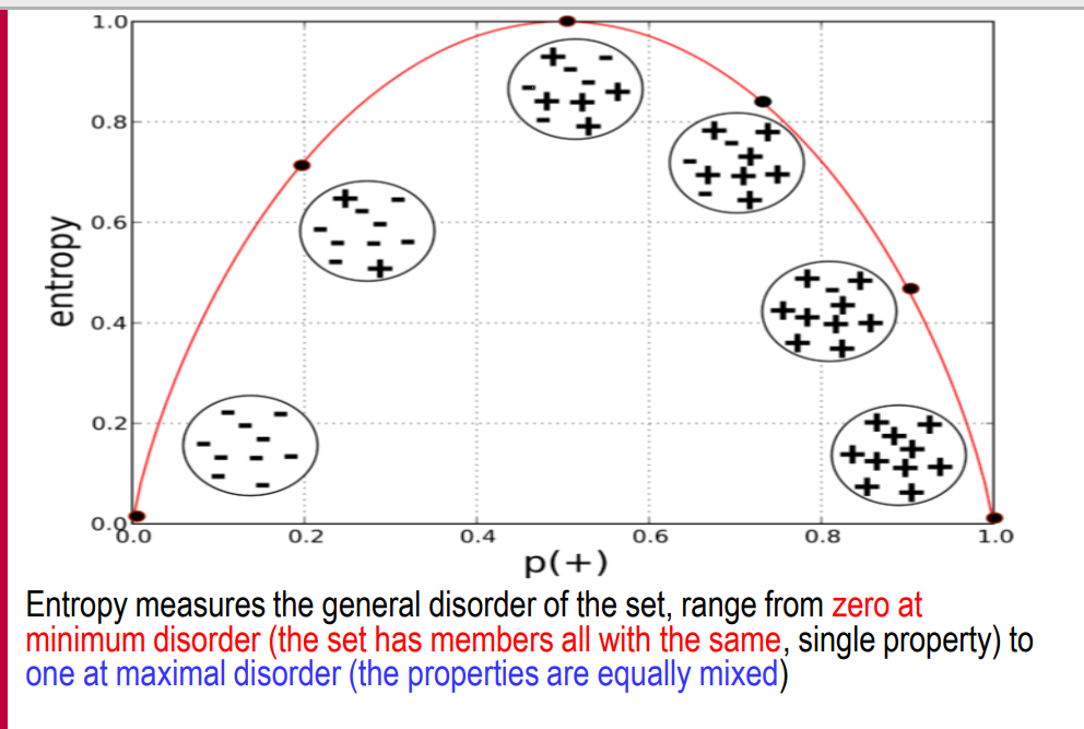
-> 엔트로피가 높을수록, 무질서가 높은 것이다.

3.2 수식

$H(X) = - \displaystyle \sum_{x \in X}p(x) log_{b}\ p(x)$

• $H(X)$는 랜덤 변수 $X$의 엔트로피
• $p(x)$는 $X$가 값 $x$를 가질 확률
• $b$는 로그의 밑으로, 보통 2를 사용하며 이 경우 엔트로피의 단위는 비트(bits)가 됩니다.

3.3 Information Gain

Entropy ,only tells us how impure one individual subset is 반면에

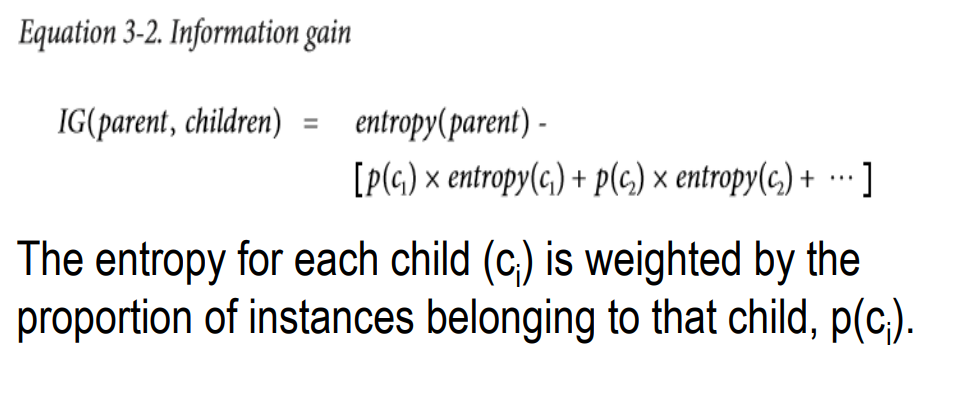
Information gain(IG) measures how much an attribute improves (decreases) entropy over the whole segmentation it creates.

• IG measures the change in entropy due to any amount of new information being added (새로운 정보의 추가에 따른 엔트로피의 변화량)

• IG is a function of both a parent set and the children resulting from some partitioning of the parent set – how much information has this attribute provided?

3.3.2 IG_Example

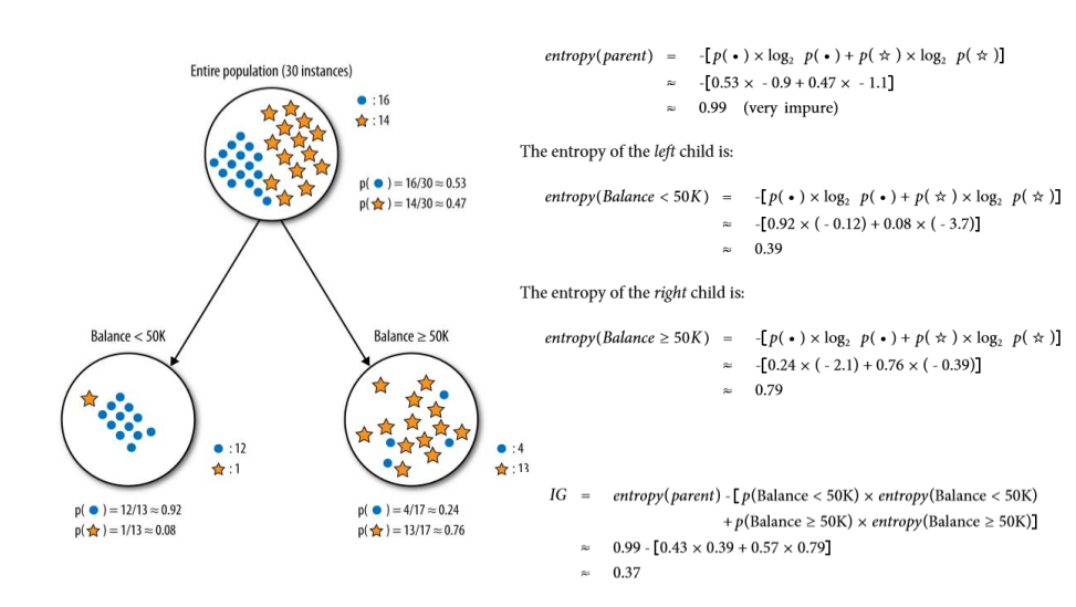
So this split reduces entropy substantially. In predictive modeling terms, the attribute provides a lot of information on the value of the target.

🤔 다르게 나눌 수 있지 않은가?
👉 나눌 수는 있다. 하지만 정보이득이 적다.정보이득이 최대가 되는 속성(attributes)찾아서 split 하는게 목표인 것이다.

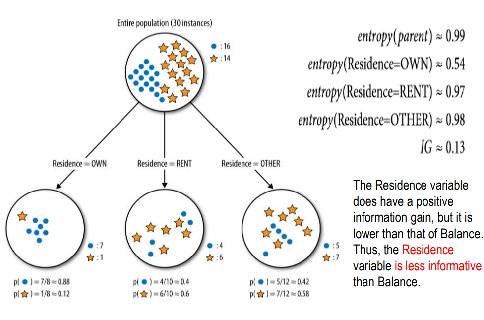
따라서
For a dataset with instances described by attributes and a target variable, we can determine which attribute is the most informative with respect to estimating the value of the target variable

🚀 We also can rank a set of attributes by their informativeness, in particular by their information gain

3.4 Mushroom Example

3.4.1 Problem situation

• This is a classification problem because we have a target variable, called edible?, with two values yes (edible) and no (poisonous), specifying our two classes
• We will use information gain to answer the question:
  “What single attribute is the most useful for distinguishing edible
  (edible?=Yes) mushrooms from poisonous (edible?=No) ones?”

3.4.2 Solved

-> IG 가 가장 높은 attribute를 골라서, 가장 좋은 속성을 선택하여 이 속성을 기준으로 edible 한지 안한지 나누어본다.

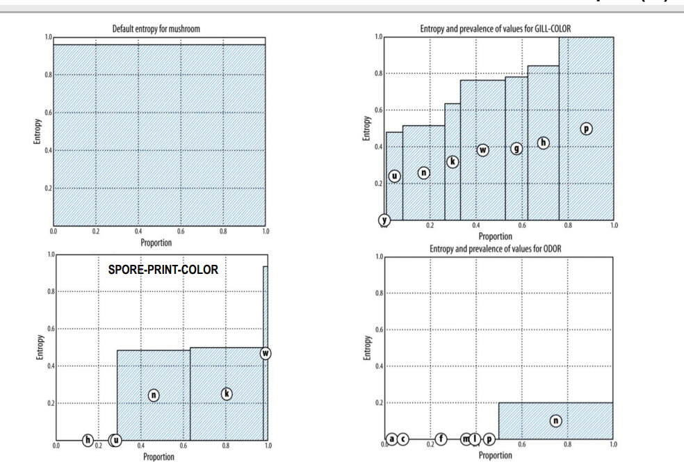
👉이 그래프들은 각 속성 값에 따라 데이터의 예측 가능성에 기여하는 정도를 엔트로피를 통해 시각화하고 있습니다. Odor 속성처럼 비율이 높고 엔트로피가 낮은 속성은 데이터의 분류에 더 도움이 될 수 있으며, 반대로 엔트로피가 높고 다양한 값이 분포한 속성은 예측에 있어 정보의 분산도가 크다는 점을 알 수 있습니다.

3.5 Supervisied segmentation with Tree-Structured Models

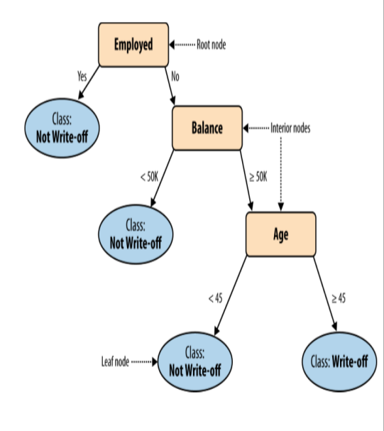
• The tree is made up of nodes,

• Each interior node in the tree contains a test of an attribute

• each path eventually terminates at a terminal node, or leaf.

Classificiation Tree

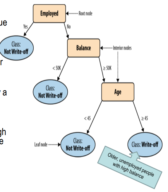
• The tree is a supervised segmentation(지도 세분화),because each leaf contains a value for the target variable.

• such a tree is called a classification tree or more loosely a decision tree.

3.6 Visualizing Segmentations

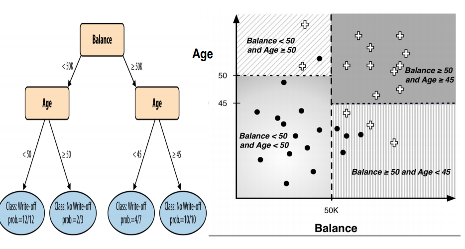
-> x축 y축으로 각 부분이 어떻게 나뉘었는지 간단하게 살펴볼 수 있는 장점이 있다.

3.7 Trees as Sets of Rules

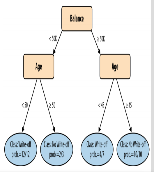
• Every classification tree can be expressed as a set of rules.

3.8 Probability Estimation

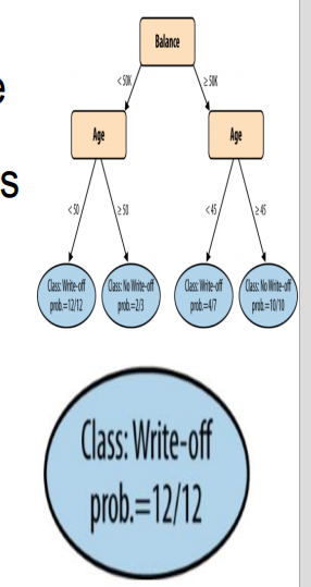
• In the context of supervised segmentation, we would like to each segment to be assigned an estimate of the probability of membership in the different classes.

4. Frequency-based estimation

If we assign the same class probability to every member of the segment corresponding to a tree leaf, we can use instance counts at each leaf to compute a class probability estimate.

A frequency-based estimate of class membership probability may be overly optimistic about the probability of class membership for segments with very small numbers of instance. (작은 샘플에 대해서는 과도하게 낙천적일 수도 있음)
<- 이를 해결하기 위해 Laplace 보정이 나타나게 함.

5. Laplace Correction

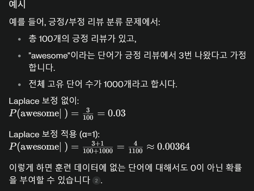
Instead of simply computing the frequency, we use a “smoothing(평활화)” version of the frequency-based estimate (Laplace correction); the purpose of which is to moderate the influence of leaves with only a few instance

Laplace 보정은 주로 나이브 베이즈(Naive Bayes) 분류기에서 사용되는 기법으로, 훈련 데이터에서 관찰되지 않은 사건에 대해 0이 아닌 확률을 할당하는 방법임.

---

Laplace 보정의 작동 방식

기본 아이디어: 모든 가능한 결과에 작은 상수값(보통 1)을 더합니다.
수식: $P(w|c) = \frac{count(w,c) + \alpha}{count(c) + \alpha K}$

여기서:
$w$: 단어
$c$: 클래스
$count(w,c)$: 클래스 c에서 단어 w의 출현 횟수
$count(c)$: 클래스 c의 총 단어 수
α: 스무딩 파라미터 (보통 1)
$K$: 고유한 단어의 총 개수

---

5.1 The Effect of Laplace Smoothing

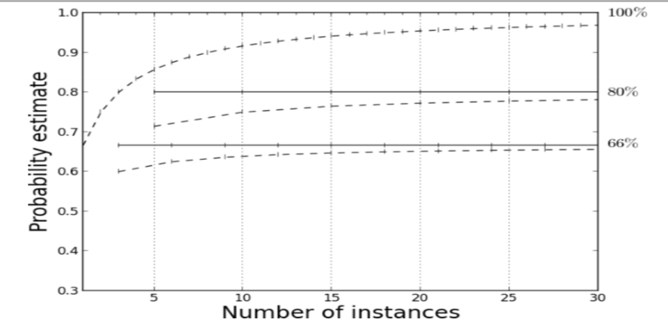
• As the number of instance increases, the Laplace equation converges to the frequency-based
  estimate.

• For each ratio the solid horizontal line shows the uncorrected (constant) estimate, while the corresponding dashed line shows the estimate with the Laplace correction applied.

• The uncorrected line is the asymptote of the Laplace correction as the number of instances goes to infinity

위 이미지 설명

긍정 100%, 80%, 66% - 실선으로 Frequency Estimation 나타내며
그 밑에 점선이 Laplace Estimation 이다.

instance 수가 적을 때, Laplace 보정은 과도한 확률을 완화하는 역할을 한다.
👉 특히 데이터의 수가 부족한 상황에서 과적합을 방지.

5.2 Example: Addressing the Churn Problem with Tree Induction

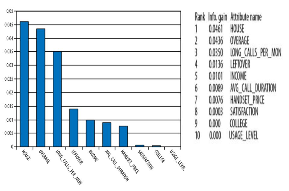
👉 Information Gain을 통해 중요한 Attributes가 무엇인지 파악할 수 있게 되었다. House와 OVERAGE 특성이 고객 특성에서 가장 중요한 요인임을 알려준다.

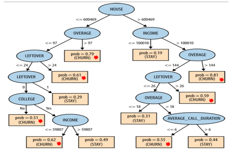
의사결정트리가 시각화되어 있다. House 의 값 600469에 따라서 첫번째 분기가 되며, 각 분기에 특성에 따라서 다시 나눌 수 있다.

6. Summary

Predictive modeling:

a model can estimate the value of a target variable for a new unseen example.
안 본 데이터에서도 predict 함

How to find and select informative attributes

– Use information gain, which is based on purity measure called entropy.
– Given a large collection of data, we can find those variables that correlate with or give us information about another variable of interest.

Tree induction

– Tree induction recursively finds informative attributes for subsets of the data.( 데이터의 하위 집합에 대해 정보를 제공하는 속성을 재귀적으로 찾습니다)

– The partitioning is “supervised” in that it tries to find segments that give increasingly precise information about the quantity to be predicted, the target.

– The resulting tree-structured model partitions the space of all possible instances into a set of segments with different predicted values for the target.(결과적으로 트리 구조의 모델은 모든 가능한 인스턴스 공간을 여러 세그먼트로 나누며, 각 세그먼트는 목표에 대한 서로 다른 예측 값을 가집니다.)

ex) 고객 이탈 예측을 한다고 가정해보자.
첫번째 분기는 소득으로 두번째 분기는 통화시간, 이렇게 하면 4가지의 세그먼트가 만들어진다.
이는 세그먼트별로 다른 이탈확률을 가지게 된다.

따라서"모든 가능한 인스턴스 공간을 나눈다"는 말은, 모든 고객 데이터를 조건에 따라 그룹으로 나누고, 그룹별로 이탈 확률 등의 예측 값을 설정하는 것을 의미합니다