0. Intro

Predictive Modeling

Predictive modeling involves finding a model of the target variable in terms of other descriptive attributes

From the data we produced both the structure of the model and the numeric “parameters” of the model

Parameter learning

• It start by specifying the structure of the model with certain numeric
  parameters left unspecified

• Then the data mining calculates the best parameter values given a particular set of training data

Assumption

① for classification and class probability estimation we will consider only binary classes

② we’re dealing with equations, this chapter assumes all attributes are numeric

③ we ignore the need to normalize numeric measurements to a common scale.

1. Classification via Mathematical Functions

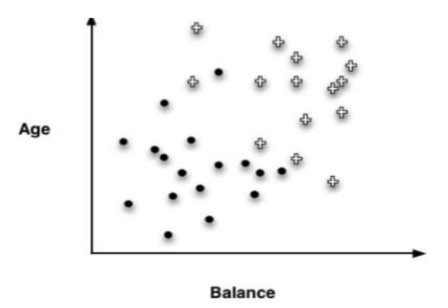
🤔 데이터가 이런 식으로 있을때, 어떻게 하면 결정경계를 '잘' 그릴 수 있을지 생각해보자.

Decision Lines

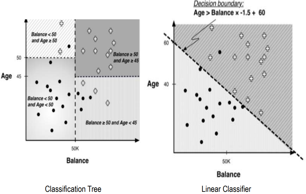
The main purpose of creating homogeneous regions is so that we can predict the target variable of a new, unseen instance by determining which segment it falls into.

It shows the space broken up into regions by horizontal and vertical decision boundaries that partition the instance space into similar regions.

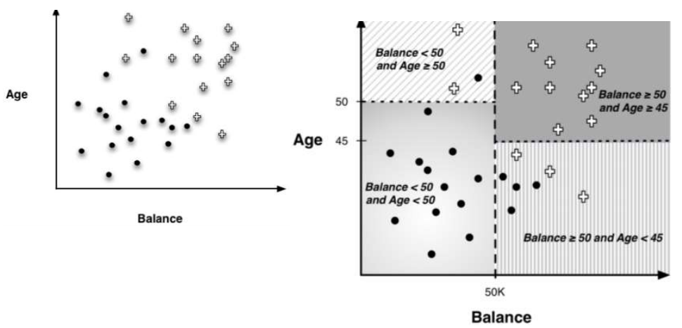
👉 위 이미지에서 보이는 바와 같이, 수평수식 decision boundaries 를 끄어서 분류 한다.

Linear Classifier

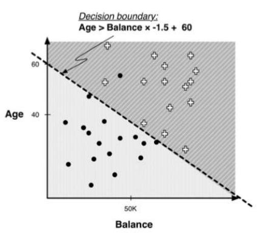
반면에 가중치의 합으로 boundary decision을 결정하는것은 linear classifier

• If we are allowed to introduce a boundary that is still a straight line, we can
  separate the instances almost perfectly.
• This is called a linear classifier and is essentially a weighted sum of the values for the various attributes

1.1 Linear Discriminant Functions

Linear discriminant(선형판별식) discriminates between the classes, and the function of the decision boundary is linear combination – a weighted sum – of the attributes.

❗ The important thing is that we can express the model as a weighted sum of the attribute values

Parameterized model

수식 : $f(x) = w_0 + w_1x_1+ w_2x_2$
$w_i$ are the parameters
-> These weights are often loosely interpreted as importance indicators of the features.
즉, The larger the magnitude of a feature’s weight, the more important that feature is for classifying the target. If a feature’s weight is near zero the corresponding feature can usually be ignored or discarded.

The Best Line for Classification

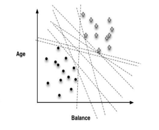
여기서 best line 은 어디일까요? -> 그걸 지금 어느 모델이냐에 따라서 다른데, 이제 3가지 모델_ SVM, linear, logistic 에 대해서 알아보자.

1.2 Optimizing an Objective Function

🤔 What should be our goal or objective in choosing the parameters?
👉 Unfortunately, creating an objective function that matches the true goal of the data mining is usually impossible,so data scientists often choose based ony faith and experience

---

기도합시다. Faith와 experience에 의존할 수 밖에 없습니다.

---

🚀 우리가 고를 수 있는 대표적인 모델들

• Support vector machine
• Linear models for regression
• Logistic regression

1.3 An Example of Mining a Linear Discriminant from Data

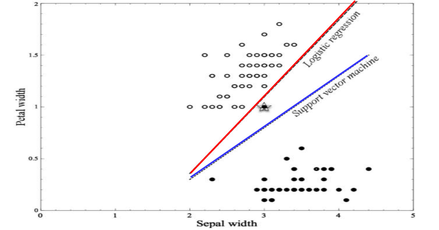
👉The methods produce different boundaries because they’re optimizing different
functions.

• Logistic 은 완전히 다 분류했지만, SVM은 잘못 분류한 것이 하나 있다.

1.4 Linear Discriminant Functions for Scoring and Ranking Instances

Which examples are more or less likely to belong to the class?
① We can build a model that produces an estimate of class membership probability.
② In the equation of the separating boundary, Equation 4-2, $f(x)$ will be zero when $x$ is sitting on the decision boundary.
③ We simply need a score that will rank cases by the likelihood of belonging to one class or the other

1.5 Support Vector Machines, Briefly

In short, support vector machines(SVMs) are linear discriminants.

SVMs classify instances based on a linear function of the features

The SVM’s objective function incorporates the idea that a wider bar is better.
-> thus the objective is the maximize the margin.

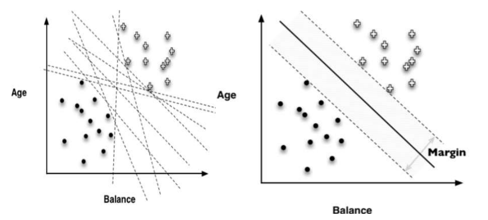
margin이 가장 큰 dash line을 선택한다.(SVM에서는)
여기서 margin이란, 결정경계와 각 클래스의 가장 가까운 데이터 포인트(서포트벡터)사이의 거리.

SVM_loss function

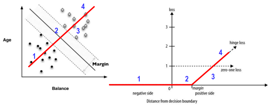
We will simply penalize a training point for being on the wrong side of the decision boundary (SVM uses hinge loss)

---

🤔hinge loss란?
📖 힌지 손실은 잘못 분류된 데이터 포인트와 마진 내에 들어온 데이터 포인트에 패널티를 부과하는 것.

---

• If the case where the data indeed are linearly separable, we incur no penalty and simply maximize the margin
• If the data are not linearly separable, the best fit is some balance between a fat margin and a low total error penalty.

2. Regression via Mathematical Functions

수식 : $f(x) = w_0 + w_1x_1 + w_2x_2 + ...$
For regression problems the target variable is numeric

• The model that fits the data best would be the model with the
  minimum sum of errors on the training data

• Standard linear regression procedures minimize the sum or mean of the squares of the errors – which gives the procedure its common name “least squares” regression.

3. Class Probability Estimation and “Logistic Regression"

Odds(승산): The odds of an event is the ratio of the probability of the event occurring to the probability of the event not occurring

<확률과 차이점>
확률은 0에서 1 사이의 숫자 또는 0%에서 100% 사이의 백분율로 표현되는 반면, odds는 유리한 결과와 불리한 결과의 비율로 표현

Odds = 유리한 결과의 수 : 불리한 결과의 수

Logistic Regression

Logistic regression uses the same linear model as do our linear discriminants for classification and linear regression for estimating numeric target values.

Log-odds linear function

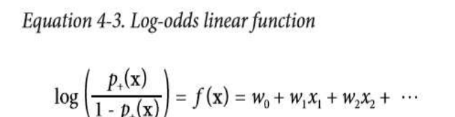
3.1 Logistic Regression: Some Technical Details

The logistic function

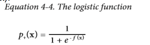
Logistic Regression Figure

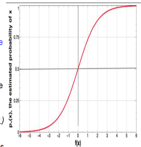
• the estimated probability p+(x) (vertical axis) as a
  function of the distance from the decision boundary (horizontal axis)
• This curve is called a “sigmoid” curve because of its “S” shape

4.4 Example: Logistic Regression versus Tree Induction

특성	분류 트리 (Classification Trees)	선형 분류기 (Linear Classifiers)
결정 경계	인스턴스 공간 축에 수직	어떤 방향이나 방향성도 가능
속성 사용	한 번에 단일 속성 선택	모든 속성의 가중치 조합 사용
접근 방식	분할 정복 접근법을 사용한 재귀적 분할	전체 공간을 관통하는 단일 결정 표면 배치
분류 방식	조각별(piecewise) 분류기	전체 공간에 대한 단일 분류
유연성	복잡한 결정 경계 생성 가능	선형 결정 경계만 생성
해석 용이성	상대적으로 해석하기 쉬움	복잡한 모델의 경우 해석이 어려울 수 있음
과적합 위험	상대적으로 높음	상대적으로 낮음
계산 복잡성	일반적으로 낮음	데이터셋 크기에 따라 다양함

Classification Tree vs Linear Classifier

5.5 Nonlinear Functions, Support Vector Machines, and Neural Networks

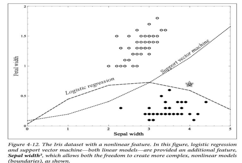
결정경계를 보면,
로지스틱 회귀는, 데이터를 분리하기 위해 특정 방향으로 기울어져 있는 반면어ㅔ
SVM은, 최대 마진을 확보하려고 하여, 로지스틱 회귀와는 다른 경계를 형성하고 있다.

6.6 Summary

• Function fitting or parametric modeling:
  -> The task of the data mining procedure is to “fit” the model to the data by finding the best set of parameters.

What exactly do we mean by best fitting the data?

① The parameters to be fit by the data mining are the weights on the attributes.

② The goodness of fit is described by an “objective function”, and each technique uses a different function.

③ The resulting techniques may be quite different.