0. Intro

We are interested in patterns that generalize (일반화 시킬 수 있는 모델에 관심) – that predict well for instances we have not yet observed

Finding chance occurrences in data that look like interesting patterns, but which do not generalize, is called overfitting the data (흥미롭지만, 일반화 시킬 수 없는 우연한 패턴의 발견은 과적합)

1. Generalization

We want models to apply not just to the exact training set (학습 데이터에만 적합한 모델이 아니라) but to the general population from which the training data came. (학습데이터의 모집단에 적합한 모델을 찾는 것이 목표)

2. Overfitting

Overfitting is the tendency of data mining procedures to tailor models to the training data, at the expense of generalization to previously unseen data points.(일반화를 희생하면서 훈련 데이터에 모델을 맞추려는 경향)
👉 There is a fundamental trade-off between model complexity and the possibility of overfitting.(모델의 복잡성과 과적합의 가능성 사이에는 trade-off 관계)
There is no single choice or procedure that will eliminate overfitting.

– The best strategy is to recognize overfitting and to manage complexity in a principled way.

3. Holdout Data = Test data

• What we need to do is to “hold out” some data for which we know the value of the target variable, but which will not be used to build the model.
• There is likely to be a difference between the model’s accuracy on the training set (sometimes called the “in-sample” accuracy) and the model’s generalization accuracy, as estimated on the holdout data.
  
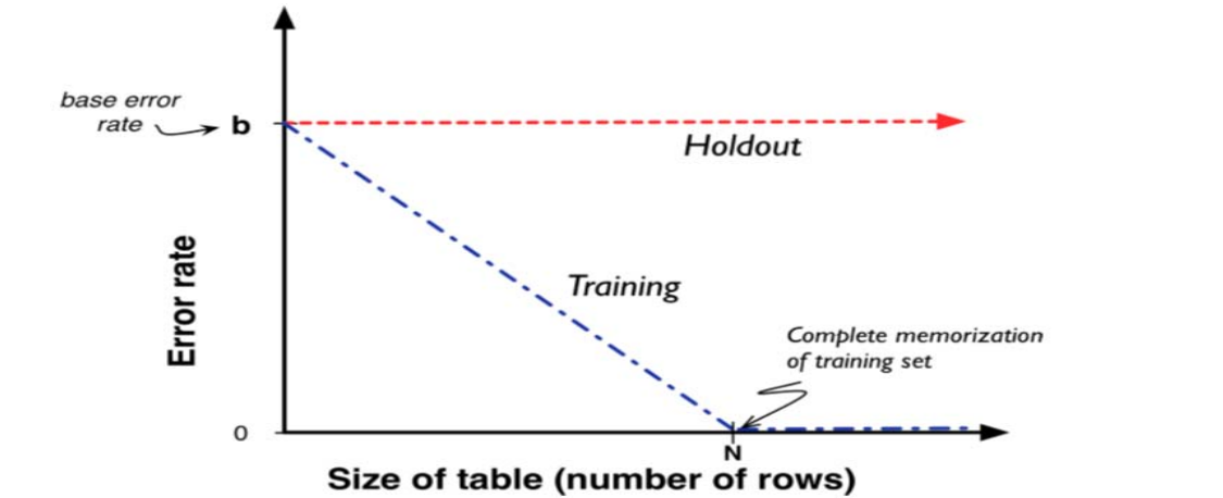
  As we allow the table to increase in size, we can memorize more and more of the training set, and with each new row the training set error decreases
• The testing (holdout) set error starts at some value (let’s call it b) and never decrease, because there is never an overlap between the training and holdout sets. => The large gap between the two is a strong indication of memorization

3.1 Holdout Data and Fitting Graphs

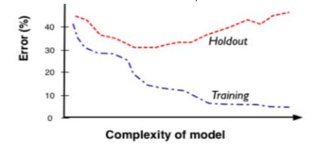
The fitting graph shows the difference between a modeling procedure’s accuracy on the training data(훈련 데이터의 정확도) and the accuracy on holdout data(테스 트 데이터의 정확도) as model complexity changes.

A Fitting Graph for Table model

👉 the table is large enough to contain the entire training set (marked N on
the x axis) and the error goes to zero and remains there.
-> The testing (holdout) set error starts at some value (let’s call it b) and never decrease, because there is never an overlap between the training and holdout sets => train 과 test간의 차이가 심함.

3.2 Overfitting in Tree Induction

• How to build tree-structured models for classification
  -> We applied a fundamental ability to find important, predictive individual attributes repeatedly (recursively) to smaller and smaller data subsets.
• If we continue to split the data, eventually the subsets will be pure all instances in any chosen subset will have the same value for the target variable.
  A procedure that grows trees until the leaves are pure tends to overfit(단말노드가 순수해 질때까지 트리를 구성하게 되면 과적합)

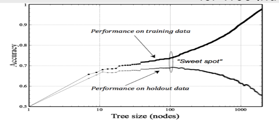
We measure two values: its accuracy on the training set and its accuracy on the holdout (test) set.
– Training-set accuracy is at least a little better than holdout-set accuracy.
– As the trees are allowed to get larger, the training-set accuracy continues to increase.

Sweet Spot
– But the holdout-set accuracy declines as the tree grows past its “sweet spot”; the data subsets at the leaves get smaller and smaller, and the model generalizes from fewer and fewer data
=> 트리의 크기(노드 수)에 대해 학습 데이터(training data)와 홀드아웃 데이터(holdout data) 사이의 성능 차이가 최소화되는 지점

4. Example : Overfitting liear functions

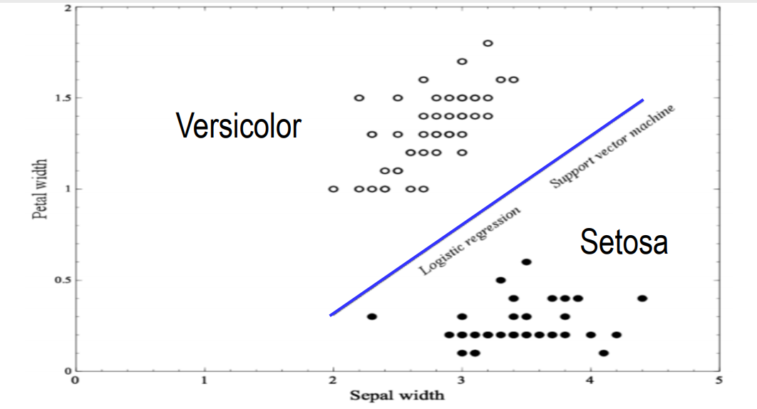
Both logistic regression and support vector machines place separating boundaries in the middle

But Outlier 가 있다면 어떨까?

Outlier of Setosa

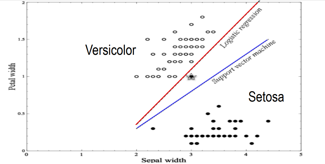
• We’ve added a single outlier of Setosa at (3,1).
• Logistic regression line moves in response: it separates the two groups perfectly.
• Support vector machine line barely moves at all.

Outlier of Versicolor

• We’ve added a single outlier of Versicolor at (4, 0.7).
• Logistic regression line moves in response: it separates the two groups perfectly.
• Support vector machine line moves very little in response.

두개의 Outlier를 보았을때 인사이트
👉 SVM이 logistic regression 보다 훨씬 덜 민감함을 알 수 있다.

Adding More Variables

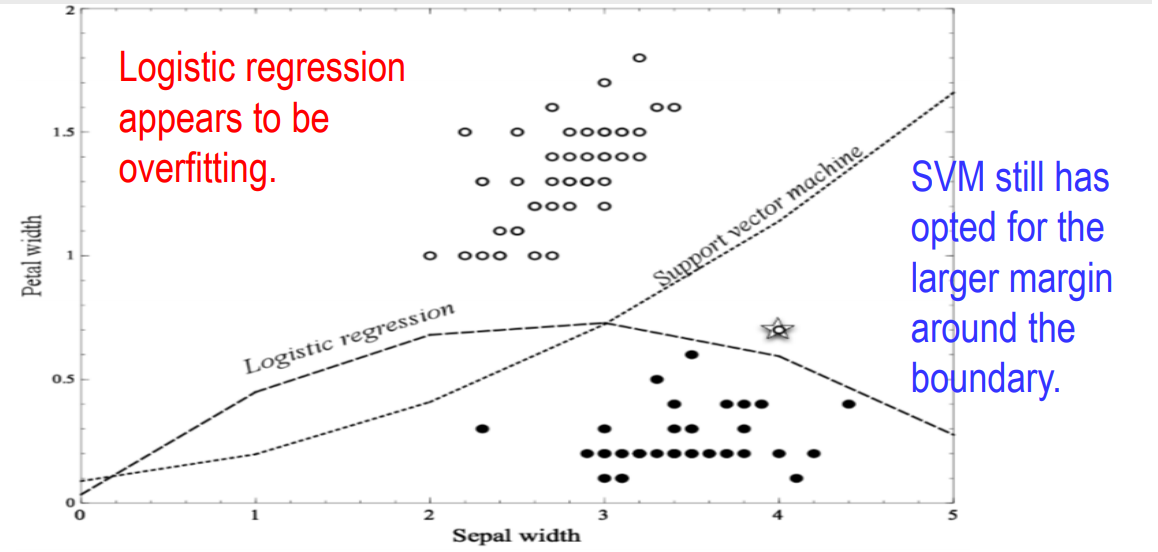
• Providing this attribute gives each model more flexibility in fitting the data.
• This additional freedom allows both methods to create curved surfaces that can fit the regions more closely.

5 Example: Why Is Overfitting Bad?

① As a model gets more complex it is allowed to pick up harmful spurious correlations(가짜 연관성까지 학습).

② These correlations are idiosyncrasies of the specific training set used and do not represent characteristics of the population in general (모집단의 특성이 아닌, 학습 데이터의 특성을 반영)

③ This harm occurs when these spurious correlations in trainingset produce incorrect generalizations in the model (학습 데이터의 가짜 연관성을 모집단의 특성으로 잘못 일반화)

④ This is what causes performance to decline when overfittingoccurs (과적합으로 인하여 성능이 하락)

6. From Holdout Evaluation to Cross-Validation

We should estimate its accuracy on holdout data.

Cross-validation is a more sophisticated holdout training and testing procedure.
– Unlike splitting the data into one training and one holdout set, crossvalidation computes its estimates over all the data by performing multiple splits and systematically swapping out samples for testing.

– Cross-validation begins by splitting a labeled dataset into k partitions called folds.

– In each iteration of the cross-validation, one fold is chosen as the test data, and the other k-1 folds are combined to form the training data.

– So, in each iteration we have (k-1)/k of the data used for training and 1/k used for testing.

– When cross-validation is finished, every examples will have been used only once for testing but k-1 times for training.

– We have performance estimates from all the k folds and we can compute the average and standard deviation.

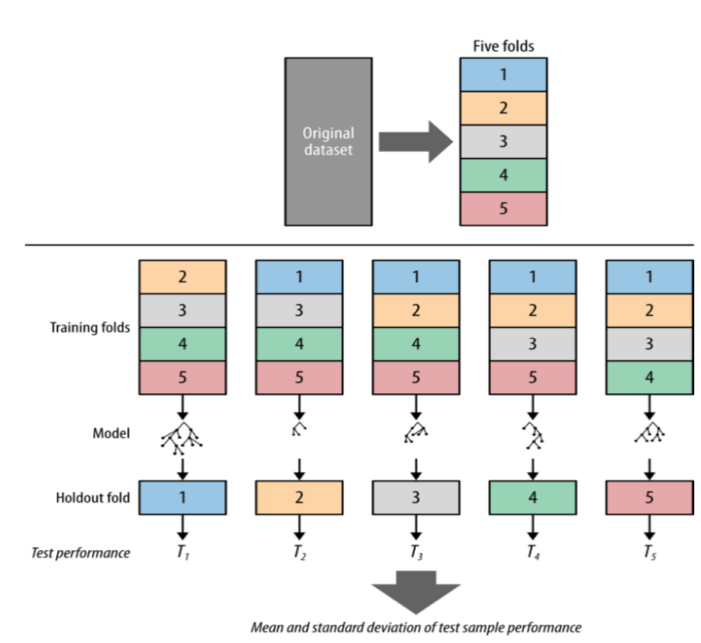
👉 The result is five different accuracy results, which then can be used to compute the average accuracy and its variance

7. Learning Curves

All else being equal, the generalization performance of data driven modeling generally improves as more training data become available, up to a point.(훈련데이터가 많을수록 모델의 성능은 향상)

A plot of the generalization performance against the amount of training data is called a learning curve(학습곡선).
다.

학습 곡선의 특징

초기 단계
초기에는 모델링 과정이 데이터셋에서 보다 명백한 규칙성을 찾아내기 때문에 급격하게 증가합니다.

중간 단계
모델링 과정이 점점 더 많은 데이터셋에서 훈련할 수 있게 되면, 더 정확한 모델을 찾게 됩니다.

후기 단계
더 많은 데이터를 사용할 때 얻는 한계적 이점은 줄어들며, 학습 곡선은 점점 덜 급격해집니다.

최종 단계
경우에 따라서는 훈련 데이터가 더 이상 정확성을 개선할 수 없기 때문에 곡선이 완전히 평평해질 수도 있습니다.

👉 이러한 특징들은 학습곡선이 데이터 양의 증가에 따른 모델 성능 향상을 어떻게 나타내는지를 보여줍니다. 초기에는 빠른 성능 향상을 보이지만, 점차 그 향상 속도가 감소하며, 때로는 더 이상의 개선이 불가능한 지점에 도달할 수 있음을 설명합니다.

Learning curves for churn problem

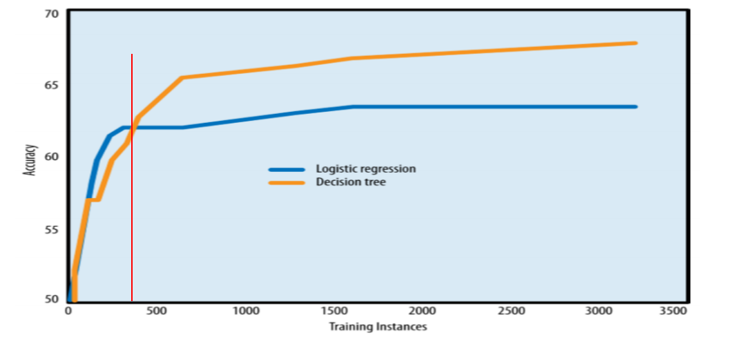
– Logistic regression has less flexibility, which allows it to overfit less with small data, but keeps it from modeling the full complexity of the data.

– Tree induction is much more flexible, leading it to overfit more with small data, but to model more complex regularities with larger training sets

Learning Curve vs. Fitting Graphs

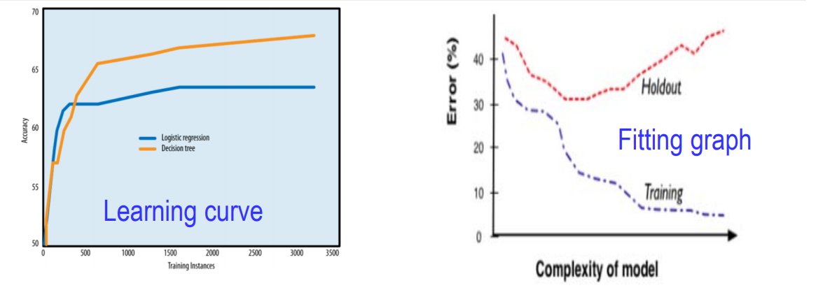
• A learning curve(학습곡선) shows the generalization performance –the performance only on testing data, plotting against the amount of training data used.

• A fitting graph(적합도그래프)(or fitting curve) shows the generalization performance as well as the performance on the training data, but plotted against model complexity. Fitting graphs generally are shown for a fixed amount of training data.

8. Overfitting Avoidance and Complexity Control

8.1 Avoiding Overfitting with Tree Induction

To avoid overfitting, we control the complexity of the models induced from the data.

Two techniques to avoid overfitting

① To stop growing the tree before it gets too complex – By specifying a minimum number of instances that must be present in a leaf (단말노드에 존재하는 사례의 최소값을 지정)

② To “prune” it back, reducing its size (and thereby its complexity).

• One general idea is to estimate whether replacing a set of leave or a branch with a leaf would reduce accuracy. If not, then go ahead and prune (가지치 기를 해도 정확도가 훼손되지 않으면 가지치기를 실행)

🤔 What threshold should we use?
👉 우연인지 아닌지 검증하기 위해서

• If the hypothesis test concludes that it was likely not due to chance, then the split is accepted and the tree growing continues.
• The hypothesis test is based on a “p-value”, which gives a limit on the probability that the difference in statistic is due to chance.
• If this value is below a threshold (often 5%), then the hypothesis test concludes that the difference is likely not due to chance.

Nested Holdout testing

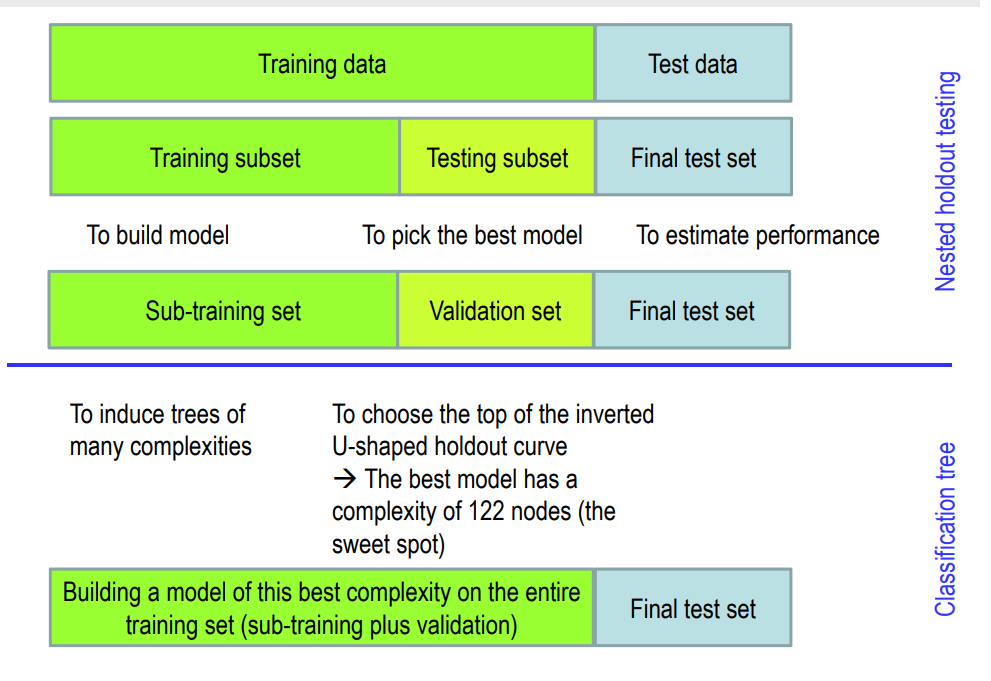
training set를 validation set 과 sub-training set로 나누어서 validation set에서 가장 좋았던 모델 선택.

8.2 A General Method for Avoiding Overfitting

Test data should be strictly independent of model building so that we can get an independent estimate of model accuracy

8.3 Avoiding Overfitting for Parameter Optimization

Avoiding overfitting involves complexity control:
finding the “right” balance between the fit to the data and the complexity of the model.(데이터에 fit 하는 것과 model의 복잡성사이에 균형을 맞추는 것)

Regularization(규칙화)

• Regularization is trying to optimize not just the fit to the data, but a combination of the fit(모델의 적합성) to the data and simplicity(모델의 복잡성) of the model.
• Models will be better if they fit the data better, but they also will be better if they are simpler.
• The general strategy is that instead of just optimizing the
  fit to the data, we optimize some combination of fit and simplicity.

Complexity Control via Regularization

Complexity control via regularization works by adding a penalty for complexity to this objective function.

• not regularization(정규화가 없을경우)

  $arg \ max_w[fit(x,w)]$

  -> The arg max $w$ just means that you want to maximize the fit over all possible arguments $w$, and are interested in the particular argument $w$ that gives the maximum.

• on regularization(정규화가 있다)

  $arg \ max_w[fit(x,w) - \lambda \ penaliy(w)]$

  The λ term is simply a weight that determines how much importance the optimization procedure should place on the penalty, compared to the data fit
  $\lambda$ 는 사용자가 정하는 변수.

9. Summary

• Data mining involves a fundamental trade-off between model complexity and the possibility of overfitting

• There is no single choice or technique to eliminate overfitting.

• A common experimental methodology called cross-validation specifies a systematic way of splitting up a single dataset such that it generates multiple performance measure

• The general method for reining in model complexity to avoid overfitting is called model regularization.

10. cf)

logistic regression 수식

수식 :
① 먼저 입력 변수를 기반으로 가중치와 편향을 사용하여,선형 결합을 계산

② 선형 결합 값 $z$를 시그모이드 함수에 입력하여 출력값이 [0,1] 사이의 확률로 변환

③ 이를 최종확률 예측하면

👉 로지스틱 회귀는 예측 확률을 출력하기 때문에, 모델이 각 클래스에 속할 가능성을 해석할 수 있다.