Business tasks involve reasoning from similar examples.

If two things (people, companies, products) are similar in some ways they often share other characteristics as well.

• Similarity can be used for doing classification and regression(분류 또는 회귀 분석에 유사성을 사용)

• We want to group similar items together into clusters (군집화)

• We use similarity to provide recommendations of similar products or from similar people (추천시스템)
  People who like X also like Y.
  Customers with your browsing history have also looked at …

• Reasoning from similar cases extends beyond business application: Case-based reasoning helps doctors and lawyers (사례기반추론)

1. Similarity and Distance

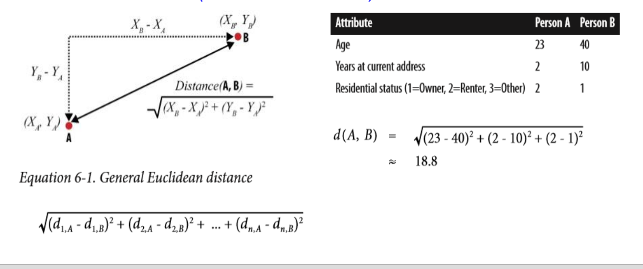
If we have two (numeric) features, then each object is a point in a two-dimensional space.

The most common geometric distance measure is called the Euclidean distance (유클리드 거리).

2. Nearest-Neighbor Reasoning

We can use similarity distance measure(유사도거리) to find the companies most similar to our best corporate customers, or the online consumers most similar to our best retail customers

These most-similar instances are called nearest neighbors(최근접 이웃)

2.1 Example: Whiskey Analytics

1단계: 위스키 비교를 위해 Color, Nose, Body, Palate, Finish 의 다섯 가지 특징을 정의한다.

2단계: Bunnahabhain의 경우 Color(gold), Nose(fresh, sea), Body(firm, medium, light), Palate(sweet, fruity, clean), Finish(full)로 특징을 요약한다.

3단계: Bunnahabhain과 다른 위스키들의 특성 차이를 수치화하여 거리(distance)로 표현한다.

4단계: 계산 결과, Bunnahabhain과 가장 비슷한 위스키는 Glenglassaugh(0.643), 그 다음은 Tullibardine(0.647), 이어 Ardbeg, Bruichladdich, Glenmorangie(0.667) 순이다.

5단계: 이 정보를 활용하여 Bunnahabhain과 유사한 맛을 가진 위스키를 선택할 수 있다

2.2 Nearest Neighbors for Predictive Modeling

Given a new example whose target variable we want to predict, we scan through all the training examples and choose several that are the most similar to the new example (훈련데이터에서 예측하고자 하는 사례와 가장 유사한 사례를 찾음)

-> Then we predict the new example’s target value, based on the nearest neighbors’ (known) target values (유사한 사례의 타겟값을 이용하여 예측 사례의 타겟값을 유추)

-> Suppose we have some combining function (like voting or averaging) operating on the neighbors’ known target values. (타겟값이 여러 개 일 경우는 평균이나 표결방식을사용)

-> The combining function will give us a prediction.

How neighbors can be used to classify a new instance?

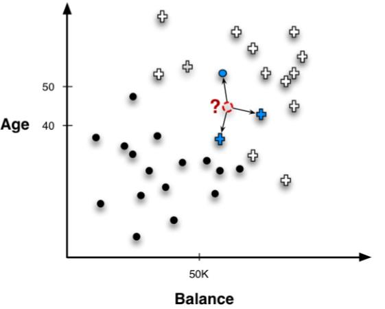
문제상황) 위에 ? 에가 어디에 속하는지를 예측하고 싶음.

The nearest neighbors (in this example, 3 of them) are retrieved and their known target variables (classes) are consulted.

– In this case, two examples are positive and one is negative.
• A simple combining function in this case would be majority vote.

– The predicted class would be positive (+, +, -).

하드보팅을 통해서 결국에는 ? 를 추측하는것임.

---

hard voting? soft voting? 에 대해서 알아보자.

하드보팅(Hard Voting)과 소프트보팅(Soft Voting) 개념

머신러닝의 앙상블(Ensemble) 기법 중 보팅(Voting) 은 여러 개의 예측 모델(분류기)로부터 나온 결과를 종합하여 최종 결과를 결정하는 방식입니다. 크게 하드보팅(Hard Voting) 과 소프트보팅(Soft Voting) 으로 나뉩니다.

하드보팅(Hard Voting)

• 각 분류기의 “최종 예측 레이블” 을 취합해서 가장 많이 나온 레이블을 최종 예측으로 채택합니다.
• 일종의 과반수 투표 방식과 유사합니다.

예시

예를 들어, 이미지가 고양이인지 개인지를 예측하는 문제에서, 세 개의 분류기가 있다고 해봅시다.

1. 분류기 A의 예측: 고양이
2. 분류기 B의 예측: 고양이
3. 분류기 C의 예측: 개

위 결과에서 가장 많이 나온 레이블은 “고양이” 이므로 하드보팅 결과는 “고양이”가 됩니다.

소프트보팅(Soft Voting)

• 각 분류기의 클래스별 확률(또는 신뢰도) 출력을 평균 해서 가장 높은 확률을 갖는 클래스를 최종 예측으로 합니다.
• 확률값이 제공되어야 하므로, 일반적으로 로지스틱 회귀나 확률적 예측을 지원하는 모델에 적용됩니다.

예시

위 예시와 동일한 분류 문제(고양이 vs 개)에서, 분류기별 확률값이 다음과 같다고 합시다.

분류기	고양이 확률	개 확률
A	0.60	0.40
B	0.80	0.20
C	0.30	0.70

각 클래스별 확률을 평균 하면 아래와 같습니다.

• 고양이 확률 평균: (0.60 + 0.80 + 0.30) / 3 = 0.57
• 개 확률 평균: (0.40 + 0.20 + 0.70) / 3 = 0.43

가장 높은 확률은 0.57 (고양이) 이므로, 소프트보팅 결과는 “고양이”로 예측됩니다.

간단 요약

• 하드보팅(Hard Voting): 분류기들의 과반수 예측 레이블 을 최종 예측으로 선택
• 소프트보팅(Soft Voting): 분류기들의 클래스별 확률값을 평균 하여 확률이 가장 높은 레이블을 최종 예측으로 선택

---

Credit Card Marketing Example

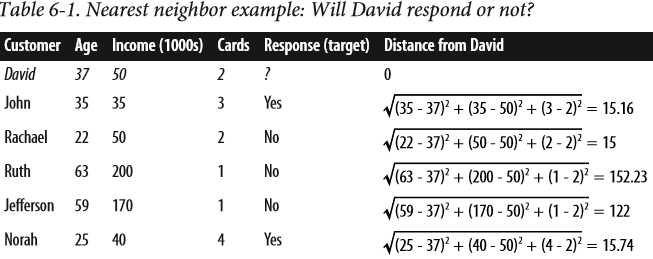
문제상황) The goal is to predict whether a new customer will respond to a credit card offer based on how other, similar customers have responded

-> If we take a majority vote, we predict Yes (David will respond)

2.3 How Many Neighbors and How Much Influence?

How many neighbors should be used?
– There is no simple answer to how many neighbors should be used.
– Odd numbers(홀수) are convenient for breaking ties for majority vote classification with two-class problems.
– In general, the greater k is the more the estimates are smoothed out among neighbors in k-NN. (k가 커질수록 추정치는 이웃과 어울림)

• Should we treat all neighbors the same?
– Intuitively, the nearest neighbors have more influence.
– Nearest-neighbor methods often use weighted voting (가중치적용 투표)or similarity moderated voting(유사도 반영 투표) such that each neighbor’s contribution is scaled by its similarity

Weighted Scoring

Weighted scoring reduces the importance of deciding how many neighbors to use.
– Because the contribution of each neighbor is moderated by its distance, the influence of neighbors naturally drops off the farther they are from the instance.

– Consequently, when using weighted scoring the exact value of k is much less critical than with majority voting or unweighted averaging (가중치 점수를 사용할 경우, k의 값에 덜 민감)
거리가 먼 이웃의 영향력이 자동으로 작아지므로, 가중치 k-NN은 k의 값에 상대적으로 덜 민감한 특징이 있습니다.

2.4 Geometric Interpretation, Overfitting, and Complexity Control

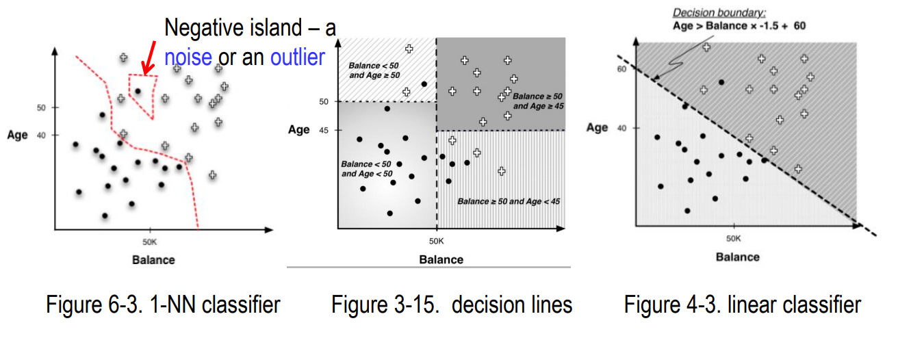
The nearest-neighbor classifier follows very specific boundaries around the training instances.
– One negative instance isolated inside the positive instances creates a “negative island” around itself. This point might be noise or an outlier.

– The 1-NN classifier predicts perfectly for training examples.

– The n-NN model simply predicts the average value in the dataset for each case.

How should one choose k?

We can conduct cross-validation or other nested holdout testing on the training set, for a variety of different values of k, searching for one that gives the best performance on the training data.

• Then when we have chosen a value of k, we build a k-NN model from the entire training set.
• Since this procedure only used the training data, we can still evaluate it on the test data and get an unbiased estimate of its generalization performance.

• Data mining tools usually have the ability to do such nested cross-validation to set k automatically.

간단 요약
(1) 여러 후보 k 값을 정한다.
(2) 훈련 세트(training set)에서 교차 검증(cross-validation) 또는 별도의 검증 세트(validation set)를 이용하여 각 k 값으로 모델을 학습·평가한다.
(3) 가장 성능이 좋은 k 값을 선택한다.
(4) 선택된 k 값으로 전체 훈련 세트를 사용해 최종 모델을 만들고, 테스트 세트로 최종 성능을 확인한다.

Different Boundaries for k-NN

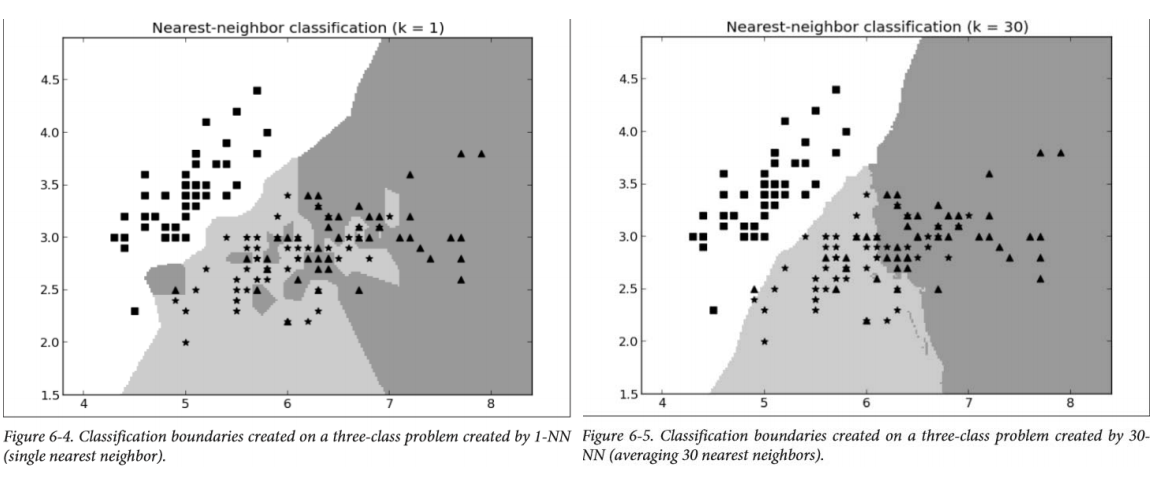
• In Figure 6-4, only a single neighbor is used, and the boundaries are erratic and very specific to the training examples in the dataset.

• In Figure 6-5, 30 nearest neighbors are averaged to form a classification and the boundaries are much less jagged.

  Note, however, that in neither case are the boundaries smooth curves or regular piecewise geometric regions that we would expect to see with a linear model or a tree structured model.

왜 경계가 울퉁불퉁(jagged)해지는가?

K=1일 때(가장 근접한 한 점만 참고)

새로운 점이 들어오면 가장 가까운 한 점만 보고 분류하므로, 훈련 데이터의 한 점 한 점이 곧 결정 경계를 뒤흔드는 역할을 합니다.
이웃이 한 명이므로, 훈련 데이터에 조금만 국소적인 변동(노이즈나 밀집)이 있어도 그 점에서 분류 경계가 불규칙하게 달라집니다.
결과적으로 훈련 데이터 포인트 “주변”만 영향을 주는 극단적인 과적합 상태가 되기 쉽기 때문에, 경계가 훈련 데이터 하나하나에 맞추어 울퉁불퉁해집니다.

K=30일 때(30개의 근접점 평균)

한 점만 보는 것이 아니라, 가장 가까운 30개의 이웃 전체를 보고 다수결(또는 평균)로 판단합니다.
단일 포인트가 주는 영향이 줄어들고, 그 주변 점들의 “집합적인” 패턴을 고려하므로 예측 경계가 좀 더 부드럽게(덜 울퉁불퉁하게) 형성됩니다.
그러나 여전히 국소적인 방식으로 데이터 분포에 의존하여 결정되므로, 선형 모델처럼 완전히 매끄러운 곡선이 되지는 않습니다.

2.5 Issues with NearestNeighbor Methods

Intelligibility

The knowledge embedded in this model is not usually understandable, so if model intelligibility and justification are critical, nearest-neighbor methods should be avoided

Dimensionality and domain knowledge

Curse of dimensionality(차원수의 저주): Since all of the attributes (dimensions) contribute to the distance calculations, instance similarity can be confused and misled by the presence of too many irrelevant attributes.

• Feature selection can be done manually by the data miner, using background domain knowledge as what attributes are relevant.

• A data scientist can tune the distance function by assigning different weights to the different attributes based on domain knowledge.

Computational efficiency

The main computational cost of a nearest neighbor method is borne by the prediction/classification step, when the database must be queried to find nearest neighbors of a new instance.

• When application requires extremely fast prediction, an nearest neighbor method may be impractical.

3. Some Important Technical Details Relating to Similarities and Neighbors

3.1 Heterogeneous Attributes

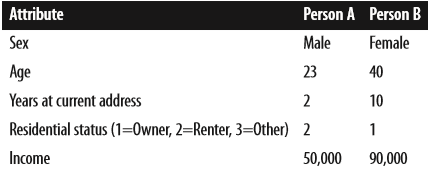
Numeric variables may have very different scales and ranges.
– Without scaling, our distance metric would consider 10 dollars of income difference to be as significant as 10 years of age difference (소득차이의 10과 나이차이의 10은 다르다)
– For this reason nearest-neighbor-based system often have variable-scaling (변수들의 단위 조정)front ends.

3.2 Other Distance Functions

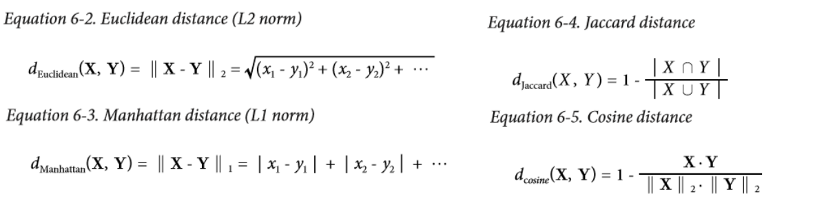
• Euclidean distance is the most widely used distance metric in data science.

• Manhattan distance simply sums the differences along the different dimensions between X and Y.

• Jaccard distance is the proportion of all, (X∪Y), the characteristics (that either has) that are shared, (X∩Y), by the two, given two objects X and Y.

- Cosine distance is used in text classification to measure the similarity of two documents.(텍스트 마이닝 적용)

Cosine Distance for Text Classification

Cosine distance is particular useful when you want to ignore differences in scale across instances – technically, when you want to ignore the magnitude of the vectors (문서의 길이는 무시)

– A = <7, 3, 2> and C = <70, 30, 20>, then dcosine(A, C) = 0 because C is simply A multiplied by 10

How Similar Two Text Fields Are?

Edit distance or the Levenshtein metric counts the minimum number of edit operations required to convert one string into the other, where an edit operation consists of either inserting, deleting, or replacing a character.
• In our two strings, the first could be transformed into the second with this sequence of operations:

1. Delete a 1,
2. Insert a c, and
3. Replace an a with an e.
   • So these two strings have an edit distance of three.

즉,레벤슈타인 거리란 두 문자열이 얼마나 다른지를 측정하는 하나의 기준인데, 최소 몇 번의 삽입/삭제/교체 연산을 통해 한 문자열을 다른 문자열로 만들 수 있는지를 숫자로 나타낸 것입니다.

주어진 예에서는 "1113 Bleaker St."를 "113 Bleecker St."로 바꾸기 위해 삭제 1회, 삽입 1회, 교체 1회 총 3번의 편집이 필요하므로, 이 두 문자열의 레벤슈타인 거리는 3이 됩니다.

4 Clustering

Clustering(군집화) is unsupervised segmentation.

• We want to find groups of objects (customers, businesses, whiskeys, etc.) where the objects within groups are similar, but the objects in different groups are not so similar.

4.2 Hierarchical Clustering

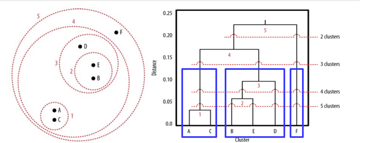
밑에서부터 올라가면서 줄여나가는 방식
In hierarchical clustering(계층적 군집화), the most general (highest-level) clustering is just the single cluster that contains everything.
즉, 최상위 군집화는 모든 것을 포함함.

위 이미지에서의 군집화는 3개로 나누면 파란색 네모처럼 나뉠 수 있음.

4.3 Nearest Neighbors Revisited: Clustering around Centroids

Hierarchical clustering focuses on the similarities between the individual instances and how similarities link them together(계층적 군집화는 개별 객체들 간의 유사도와 유사도가 객체를 서로 연결하는 방법에 초점)

In k-means clustering, the most popular centroid-based clustering algorithm, the “means” are the centroid, represented by the arithmetic means (averages) of the values along each dimensions for the instances in the cluster.

The k in k-means is simply the number of clusters that one would like to find in the data.
– Unlike hierarchical clustering, k-means starts with a desired number of clusters k. (k-평균 군집화에서는 k를 먼저 정하고 시작)

k-means Algorithm

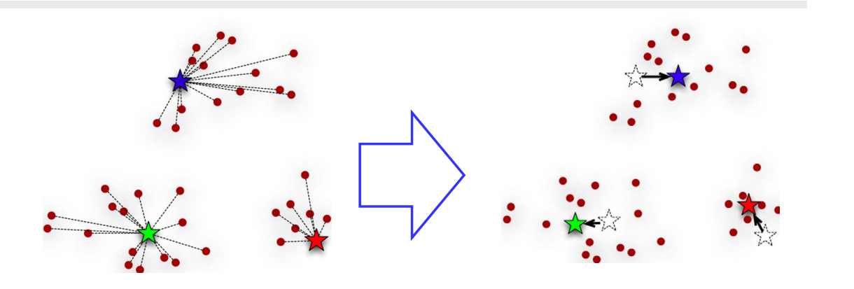
The algorithm starts by creating k initial cluster centers, usually randomly.(임의의 중심점 선정)

-> The clusters corresponding to these cluster centers are formed by determining which is the closet center to each point (중심점에 가깝게 군집화)

-> Next, for each of these clusters, its center is recalculated by finding the actual centroid of the points in the cluster. The cluster centers typically shift (군집의 중심점 재계산)

-> Since the cluster centers have shifted, we need to recalculate which points belong to each cluster(새로 군집화하고 군집의 중심점 재계산)

-> The k-means procedure keeps iterating until there is no change in the clusters (or possibly until some other stopping criterion is met.) (변동이 없을 때까지 반복)

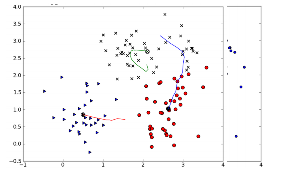
ex) k=3일때

local optimum problem

There is no guarantee that a single run of the k-means algorithm will result in a single clustering.

The result of a single clustering run will find a local optimum

For this reason, k-means is usually run many times,starting with different random centroids each time. (부분 최적화를 방지하기 위해서 시작점을 다르게 해서 여러 번 반복 수행)
–

• The clustering with the lowest distortion value can be deemed the best clustering.
• The cluster distortion is the sum of the squared differences between each data point and its corresponding centroid.

How to determine a good value for k?

One answer is simply to experiment with different k values and see which ones generate good results

For a more objective measure, the analysts can experiment with increasing values of k and graph various metrics of the quality of the resulting clusterings.

4.4 Example: Clustering Business News Stories

4.5 Understanding the Results of Clustering

How to understand clusterings and clusters depends on the sort of data being clustered and the domain of application

The general strategy is this: we use the cluster assignments to label examples
– Each example will be given a label of the cluster it belongs to, and these can be treated as class labels.

– Once we have a labeled set of examples, we run a supervised learning algorithm on the example set to generate a classifier for each class/cluster.

– We can then inspect the classifier descriptions to get a intelligible and concise description of the corresponding cluster. These will be differential descriptions

“비지도 학습 → 라벨링(클러스터 ID) → 지도 학습 적용”의 프로세스를 통해 각 클러스터(클래스)가 어떤 특징에 의해 분류되었는지를 해석 가능한 규칙(classifier description)으로 얻을 수도 있습니다.

5 Stepping Back: Solving a Business Problem versus Data Exploration

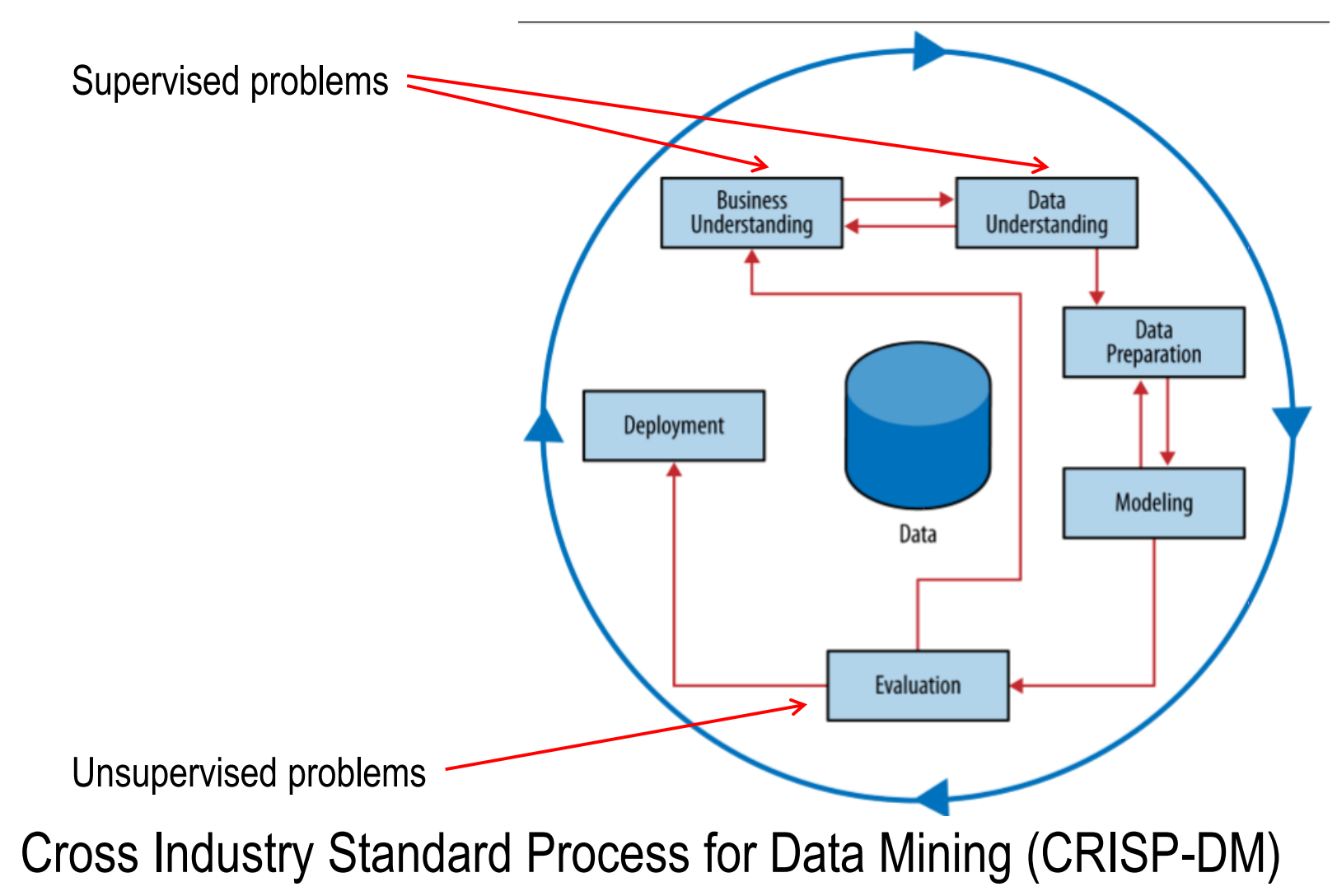
For supervised problem (such as predictive modeling), since we spent so much time defining precisely the problem we were going to solve, in the Evaluation stage we already have a clearcut evaluation question.

For unsupervised problem (such as clustering), since we did not achieve a precise formulation of the problem in the early stages, we have to spend more time later in the process – in the Evaluation stage.

6. Summary

1. 유사성은 데이터로부터 유사한 개체를 찾거나, 예측 모델링 및 군집화에 활용될 수 있다.

2. 개체 간 거리(distance)는 피처 벡터 공간에서 유사성을 추정하는 대표적인 방법이다.

3. 최근접 이웃 방법은 새로운 데이터와 기존 학습 데이터 간의 유사도 측정을 통해 예측을 수행한다.

4. 비지도 학습 방식에서는 초기 비즈니스 이해보다는 이후 평가와 반복 과정에 더 많은 시간이 든다.

유사성(similarity)은 분류, 회귀, 군집화 등 여러 기법에 사용되며, 최근접 이웃(k-NN)은 거리를 활용한 대표적인 예측 방법.
비지도학습(예: 군집화)은 체계적 문제 정의가 어렵기 때문에, 최종 평가 단계에서 해석과 탐색이 더 많이 필요하다.