1. Semantic Segmentation

1.1 What is semantic Segmentation?

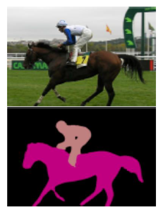
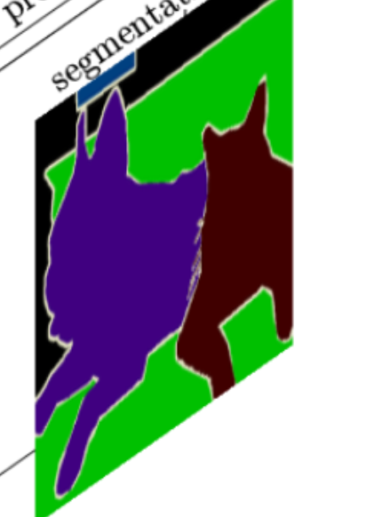
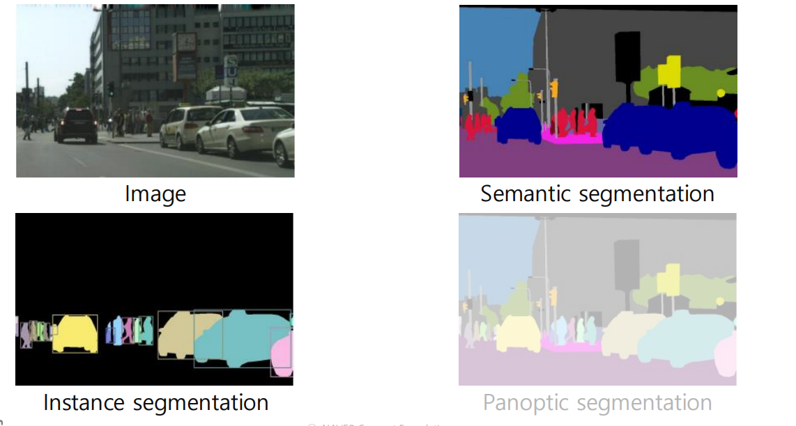
📖 Semantic Segmentationis a deep learning algorithm that associates a label or category with every pixel in an image. 즉, 위의 이미지처럼 모든 픽셀에다가 라벨붙임.

1.2 Where can semantic segmentation be applied to?

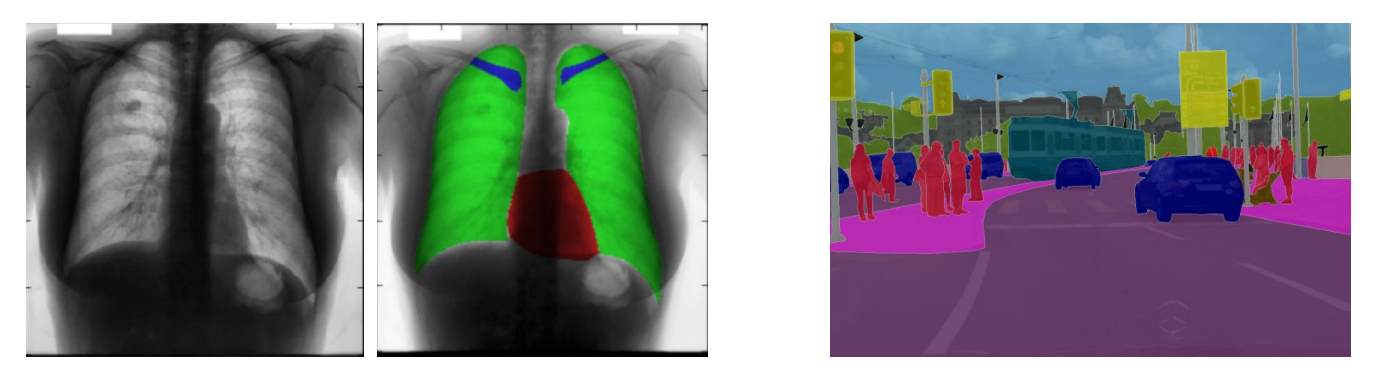
📖 영상의료나 자율주행차량에다 사용할 수 있음.

2.Semantic segmentation architectures

2.1 FCN(Fully Convolutional Networks

https://www.cv-foundation.org/openaccess/content_cvpr_2015/papers/Long_Fully_Convolutional_Networks_2015_CVPR_paper.pdf

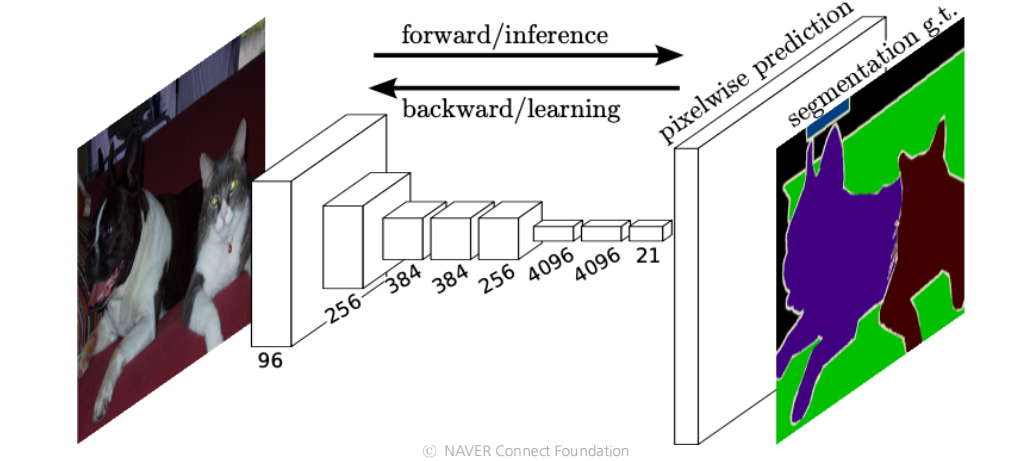
• 처음으로 end-to-end 형식의 semantic segmentation 임.
• output 에 아무형식의 사이즈(arbitrary size)넣고 output에 input size 에 대응되는(corresponding_) 사이즈 segmentation map출력

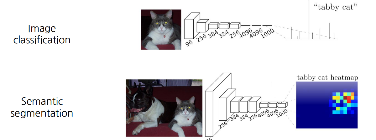
• Fully connected layer: fixed dimensinal vector and discard spatial coordinates
• Fully convolutional layer: output a classification map which has spatial coordinates
  

📖 Fully Convolutional Network의 문제점은 , 예측된 스코어 맵은(predicted score map)은 매우 낮은 해상도를(in a very low resolution)을 가진다는 점이다.

🤔 왜 낮은 해상도를 가질까?

✍️ 넓은 수용범위를 가지면(For having a large receptive field) 여러개의 공간풀링 레이어가 있기 떄문이다.
즉, 평균풀링이나 맥스풀링을 반복하면 당연히 차원이 낮아지고 이로 인해 low resolution을 가질 수 밖에 없다.

👉 Solution: Enlarge the Score map by upsampling!

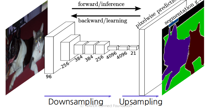
📖 Upsampling!은 small activation map을 input image 에 맞게 resize 함

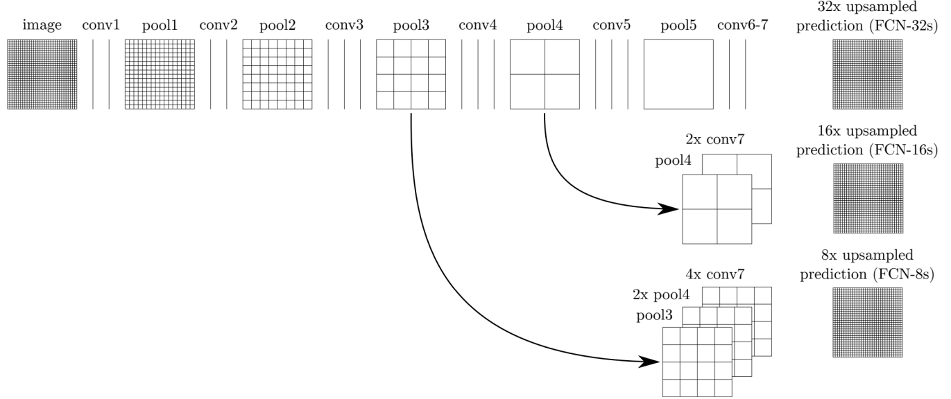
📖 위에 보이는 것처럼 skip connection을 통해 score map을 확장(enlarge)시킴!

2.2 U-Net

:https://arxiv.org/abs/1505.04597

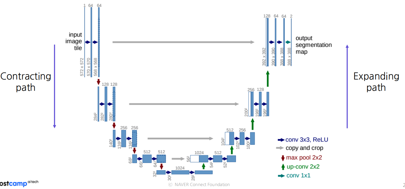
왼쪽의 Contracting Path

• 3 x 3 convolution을 반복적으로 적용
• feature channels을 2배로 함 (doubling)
• holistc context(전체적인 상황이나 관계를 고려하여 정보 이해) 를 파악할려고 사용

오른쪽의 Expanding Path

• 2 x 2 convolutional 을 반복적으로 적용함.
• feature channel수를 반으로 계속 줄임
• 왼쪽의 Contracting Path 로부터 corresponding feature map을 concatenate 함.-> 이는 지역적 정보를 주기 위함임(provide localized information)

3. Object detection

3.1 What is object detection?

객체탐지란, 디지털 이미지와 비디오로 특정한 계열의 시맨틱 객체 인스턴스를 감지하는 일

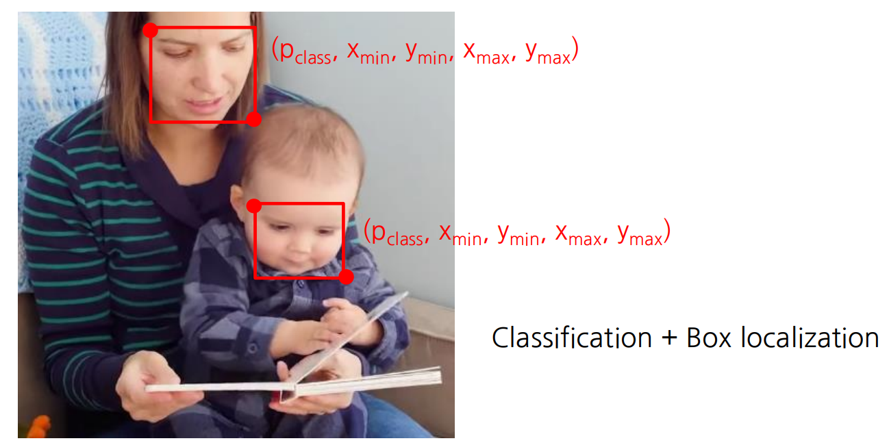
위의 예제에서 보이는 것처럼 Classification 하고 어디인지 Box localization 함.

3.2 What are the applications of object detection?

Antonomous Driving , OCR(Optical Character Recongnition)등등

4. Object detection architectures

4.1 Two-stage detector: R-CNN(Region-CNN)

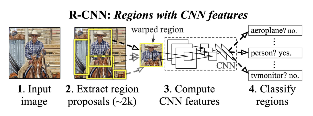
📖 순서는 이렇다
① Input Image 를 넣는다.
② Region Proposal 를 2,000 개 정도 뽑는다
③ CNN features 를 엄청나게 계산한다.
④ Classify 함.

R-CNN family

4.2 One-stage detector: YOLO(You Only Look Once)

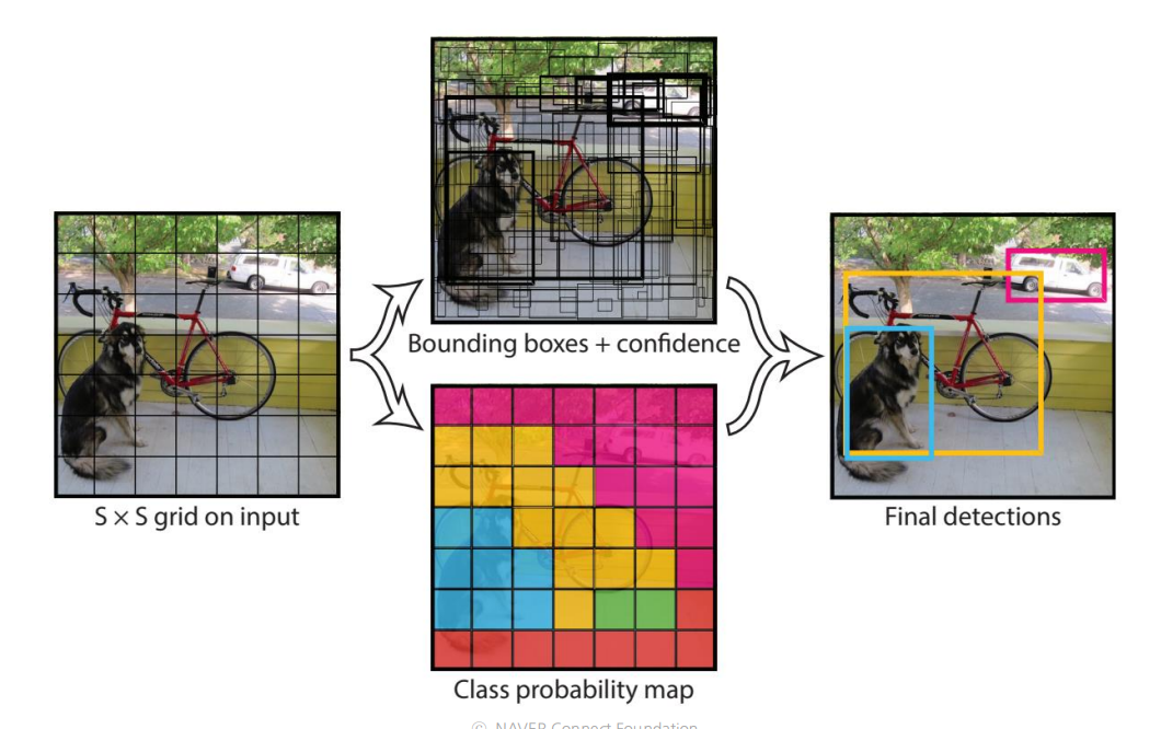
📖 지역을 추출하고 -> classifiy 하는 R-CNN과는 다르게, YOLO 는 탐지와 동시에 분류한다.
YOLO Acrhitecture

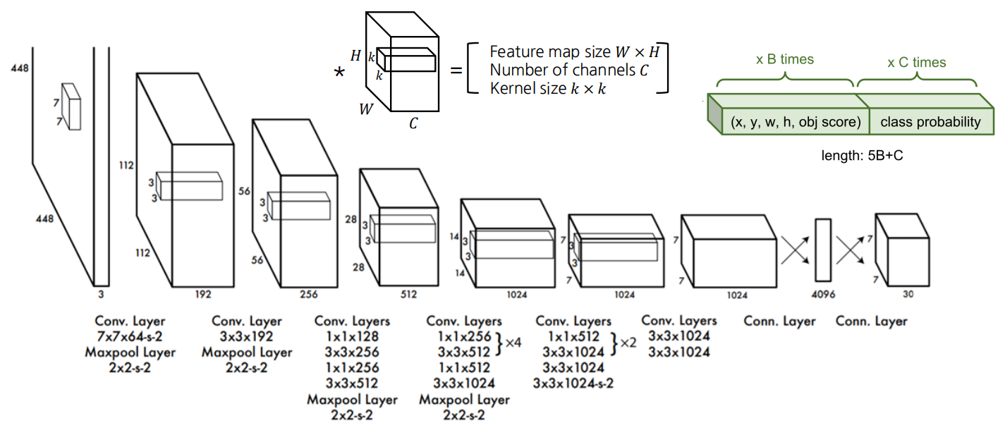
• 24 개의 convolutional layer ,4개의 max-pooling layer , 2개의 FC
• Resize input image into 448 x 448 before going convolutional layer
• 1 x 1 convolutional lyaer 가 채널의 수를 줄이기 위해 처음에 적용되고 그후에 직사각형 output 을 만들어내기위해 3 x 3 convolutional layer 를 사용함
• 정규화를 위해 batch normalization, dropout,등을 사용함.

4.3 One-stage detector vs. Two-stage detector

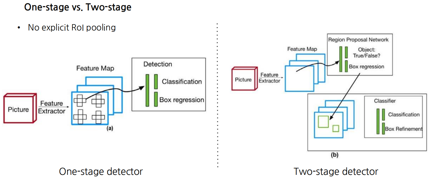
one-stage는 classificatino 과 box regression이 동시에(YOLO),
two-stage는 classification 과 box regression 이 각각.(R-CNN)

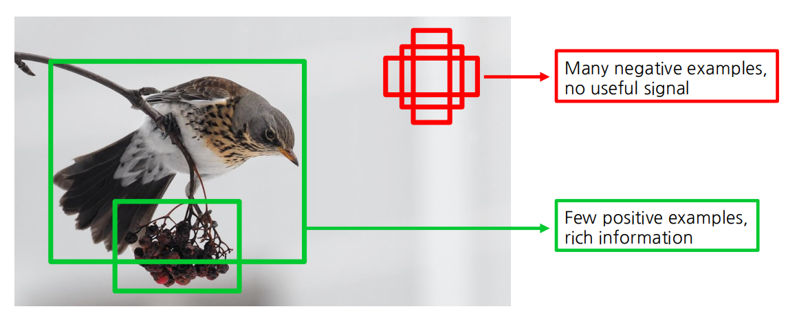
One-stage(YOLO 모형)은 긍정적인 앵커박스(객체있는거)와 부정적인 앵커박스(배경)간의 불균형이 심하기 때문에 클래스 불균형(class imbalance)가 발생한다.

이를 해결하기 위해 새로운 손실함수 Focal loss를 제안한다.

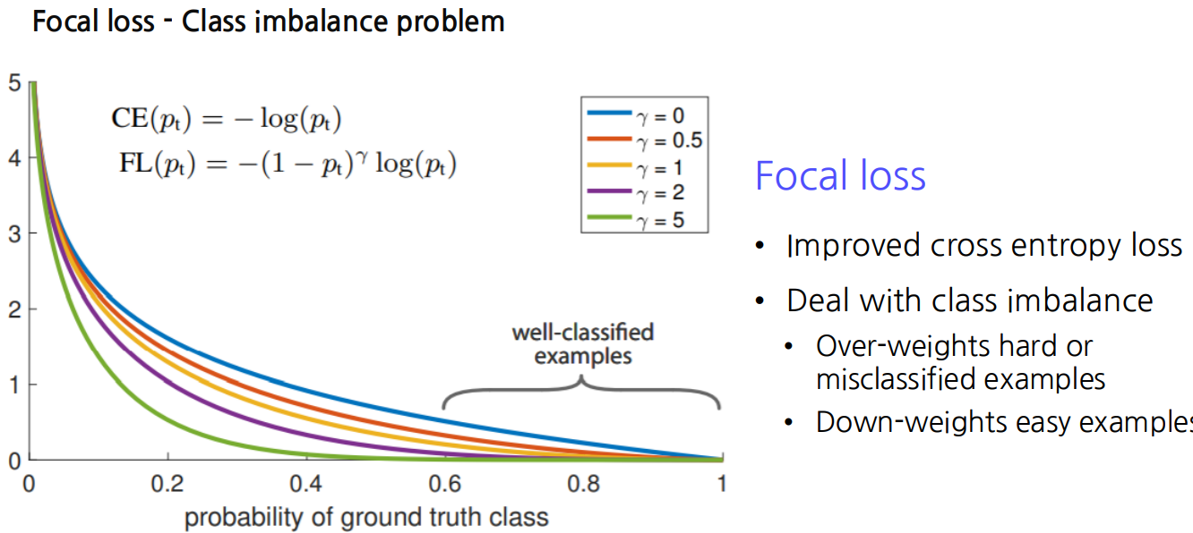
Focal loss란?

$FL(p_t) = -\alpha_t(1 - p_t)^{\gamma} \ log(p_t)$

식 해석:
① $p_t$: 정답 클래스에 대한 모델의 예측 확률
② $\alpha_t$: 클래스의 균형을 맞추기 위한 파라미터 -> 클래스 불균형을 조정하는데 사용
③ $\gamma$ : "초점"파라미터로, 모델이 어려운 샘플에 더 집중하도록 도움.

주요특징
① Easy Examples의 손실 감소:
-> $(1-p_t)^\gamma$ 항이 쉬운 샘플의 손실 기여를 줄임. 즉, 이미 틀린거 $(1-p_t)$에 모델이 더 집중하게끔함.
② Hard Examples의 손실 증가:
-> $-log(p_t)$ 항이 잘 분류한거에 마이너스를 주어서 더 틀린거에 집중하게끔함.
③ 클래스 불균형 처리
-> $\alpha_t$를 사용하여 클래스의 비율에 따라 손실을 조정할 수 있어, 클래스 불균형 문제를 완화할 수 있다.

위 Class Imbalance 문제를 Focal loss 로 푼게
RetinaNet

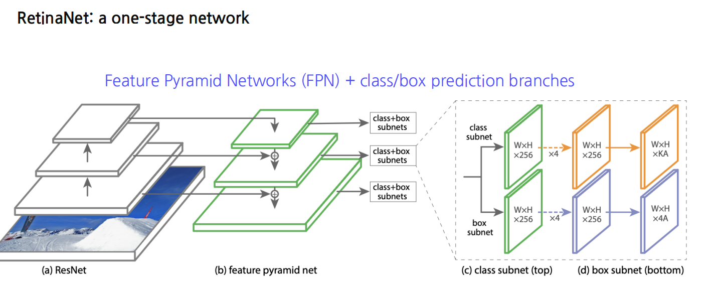
-> 논문참조.

5. Instance segmentation

5.1 Instance segmentation

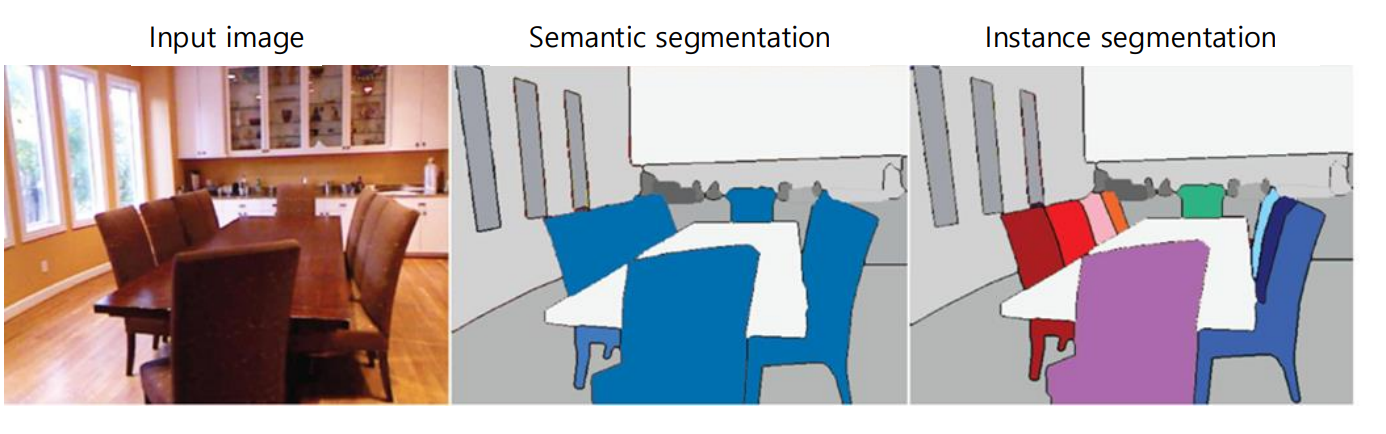
Instance Segmentation = Semantic Segmentation + distinguishing instances
📖 즉, instance segmentation은, 이미지 내의 각 개체를 개별적으로 구분하고 분할하는 고급이미지 처리 기술이다.

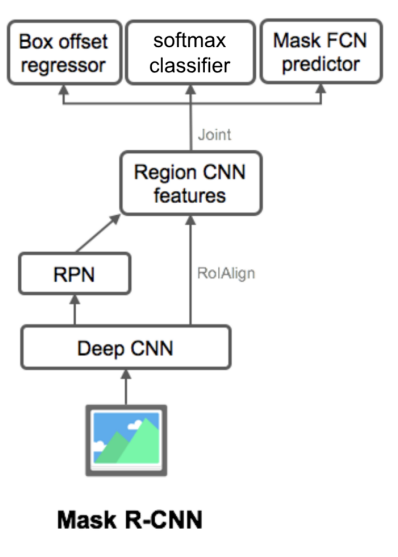
ex) Mask R-CNN, Mesh R-CNN, DensePose R-CNN등이 있다.

Mask R-CNN

6. Transformer-based methods

6.1 Extending transformers to computer vision

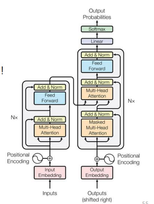
📖 Transformer 는 Attention 만 있는 구조로 이로 인해 NLP 에서 크게 성공을 거두었는데 이를 Computer Vision 에도 쓰자는게 핵심이다.

6.2 DETR(DEtection TRansformer)

DETR : End-to-End Object Detection with Transformers

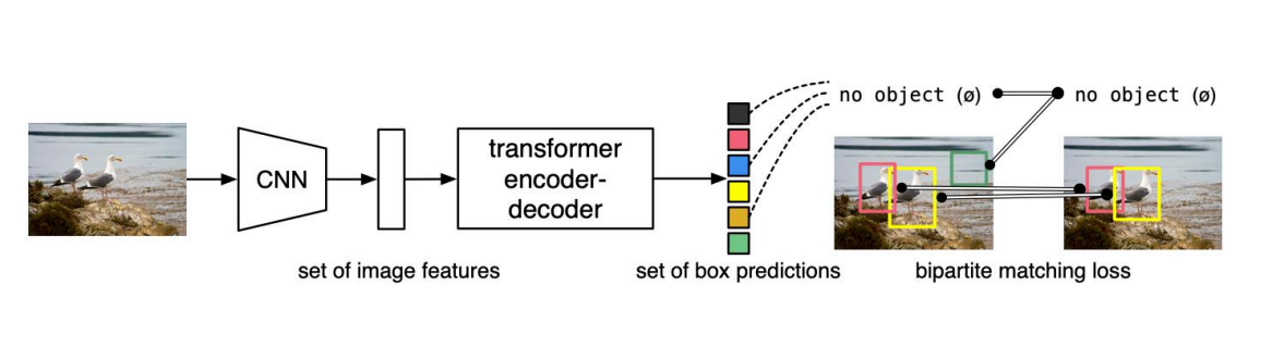
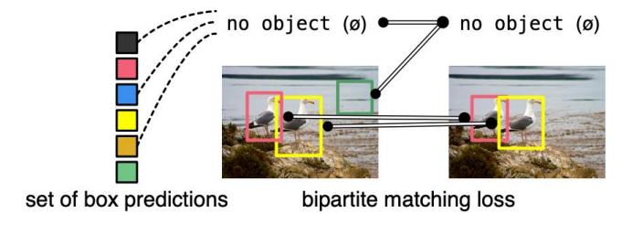
DETR directly predicts (in parallel) the final set of detections by combining a common CNN with a transformer architecture. During training, bipartite matching uniquely assigns predictions with ground truth boxes. Prediction with no match should yield a "no object"$(\phi)$ class prediction

📖DETR 특징

• Object Detection 을 직접 집합 예측 문제(direc set prediction problem)로 간주한다.
• 많은 hand-designed components를 제거했음

🤔 직접 집합 예측 문제(direct set prediction problem)이 뭐야??

👉 직접 집합 예측 문제란, 모델이 입력 데이터에서 객체들을 직접적으로 집합 형태로 예측하는 문제를 의미함. 즉, 모델이 이미지 내의 모든 객체를 한 번에 모두 찾아내고 그객체들의 위치와 종류를 동시에 예측함. -> 중간단계가 사라짐.

DETR 방법론
[1]

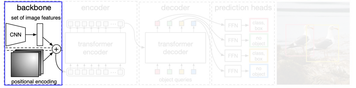
• Backbone 은 전통적인 CNNs 임
• 컴팩트한 특징표현들을 추출해냄 $f \in \mathbb R^{C \times H \times W}$
• Positional encoding을 transformer encoder에 지나기전에 더해줌

[2]

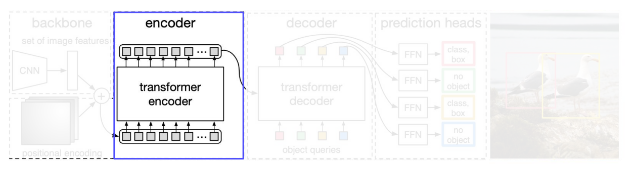
Transformer encoder

• 1 x 1 convolution 을 쓰면서, 새로운 피처 맵을 만든다. $C$ -> 더 작은 차원 $d$로
• feature map 은 $d \times HW$로 reshape함
• Fixted positional encoding을 추가함. 왜냐하면 self-attention은 permutation - invariant 하기 떄문이다. (permutation invariants란, 입력벡터 요소의 순서와 상관없이 같은 출력을 생성한다는 뜻)

[3]

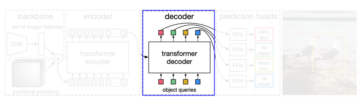
Transformer Decoder

• input -> (1) encoder outputs + (2) object queries(Learnt Positional Encoding)
  Object queries : 객체 쿼리. 이 객체쿼리는 사전에 정의된 것이 아니라, 학습가능한 위치 인코딩을 포함함.
• 각각 decoder layer 에 병렬적으로 N objects 가 decodes 함.

[4]

Prediction Heads

• $N$개의 bounding boxes 를 예측함 (당연히 $N >>$실제 objects갯수)
• 그럼 $N$이 남는게 있으니까 남는거는 label $\phi$를 써서 No object 라는 것으로 명시함.(이는 background class 와 비슷)

[5] 여기는 수식을 꼼꼼히 살펴보자.

Bipartite matching(이분 매칭)

• $y$ : Ground truth sef of objects(실제 객체의 집합)
• $\hat y = \{\hat y\}^N_{i=1}$ : set of N predictions(모델이 예측한 N개의 바운딩 박스)
• $\mathcal L_{match}$ : pairwise matching cost(매칭 비용을 측정하는 함수)
• $\sigma \in \mathfrak S_N$ : matching permutation of $N$ elements(N개의 예측 바운딩 박스와 N개의 실제 객체간의 매칭순서를 나타내는 순열,$\mathfrak S_N$은 N개의 원소로 구성된 모든 가능한 순열의 집합. )

  ① $\ \hat\sigma = arg \ min_{\sigma \in \mathfrak S_N} \displaystyle \sum^N_i \mathcal L_{match}(y_i, \hat y_{\sigma(i)})$

② $\mathcal L_{match}(y_i,\hat y_{\sigma(i)}) = \mathbb I_{c \neq\phi}\hat p_{\hat \sigma(i)}(c_i) +\mathbb I_{\{c_i \neq \phi\}}\mathcal L_{box}(b_i, \hat b_{\hat \sigma(i)})$

③ $\mathcal L_{box}(b_i, \hat b_{\sigma (i)}) = \lambda_{iou} \mathcal L_{iou}(b_i, \hat b_{\sigma(i)}) + \lambda_{L1}\parallel b_i -\hat b_{\sigma(i)}\parallel_1$

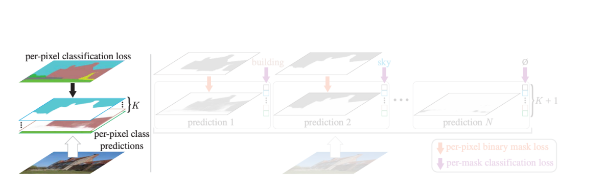
6.3 MaskFormer

MaskFormer: Per-Pixel Classification is Not All You Need for Semantic Segmentation

6.4 Uni-DVPS(Unified Model for Depth-Aware Video Panoptic Segmentation)

7. Segmentation foundation model

7.1 SAM(Segment Anything Mode)

7.2 Grounded-SAM(Grounding DINO + SAM)