
1. LSTM 개요
1-1. LSTM
LSTM(Long Short-Term Memory)은 RNN(Recurrent Neural Network)의 한 종류로, 시계열 데이터의 장기 의존성을 효과적으로 학습할 수 있도록 설계된 신경망이다. 기본 RNN이 가지는 기울기 소실(Gradient Vanishing) 문제를 해결하기 위해 고안되었다. 즉, 일반적인 RNN은 장기 기억 성능이 좋지 않으나, LSTM에서는 이 부분이 개선되었다.
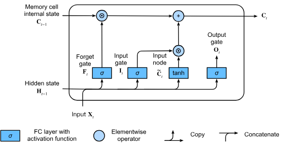
LSTM은 셀 상태(cell state)와 세 가지 게이트(입력 게이트, 망각 게이트, 출력 게이트)를 사용하여 정보의 흐름을 조절할 수 있다. (이전 정보를 잊을지 말지 판단하면서, 필요한 정보만 다음 시각으로 계승 가능하다)
1-1. LSTM 구조
LSTM Layer는 다음 구조로 이루어져 있다.
- 기억 셀(Memory cell) : LSTM은 셀 상태를 통해 장기 의존성을 유지한다. 셀 상태는 일종의 메모리 역할을 하여 중요한 정보를 장기간에 걸쳐 유지하게 된다.
- 입력 게이트(Input gate) : 새로운 정보(새로 입력되거나, 한 단계 전의 출력)가 기억 셀에 얼마나 반영될지 결정한다.
- 망각 게이트(Forget gate) : 기억 셀의 내용을 어느 정도로 남길지 조정한다. 이전 기억 셀의 정보 중 어느 부분을 잊을지 결정한다.
- 출력 게이트(Output gate) : 새로운 정보가 기억 셀에 어느 정도로 출력에 반영될지 결정한다.
LSTM 셀의 각 시간 단계에서는 다음과 같은 작업이 이루어진다.
❶ 망각 게이트 (Forget Gate)
이전 셀 상태에서 어떤 정보를 잊을지 결정한다.
❷ 입력 게이트 (Input Gate)
- 새로운 정보를 어느 정도 업데이트할지 결정한다.
- 새로운 후보 메모리 셀 상태를 생성한다.
❸ 셀 상태 업데이트 (Cell State Update)
- 셀 상태를 업데이트한다.
❹ 출력 게이트 (Output Gate)
- 셀 상태의 어느 부분이 출력될지 결정한다.
- 최종 출력을 생성한다.
2. 간단한 LSTM 구현
2-1. 훈련용 데이터 작성하기
import numpy as np
import matplotlib.pyplot as plt
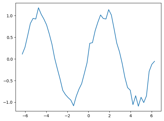
x_data = np.linspace(-2*np.pi, 2*np.pi)
sin_data = np.sin(x_data) + 0.1*np.random.randn(len(x_data))
plt.plot(x_data, sin_data)
plt.show()
n_rnn = 10
n_sample = len(x_data)-n_rnn
x = np.zeros((n_sample, n_rnn))
t = np.zeros((n_sample, n_rnn))
for i in range(0, n_sample):
x[i] = sin_data[i:i+n_rnn]
t[i] = sin_data[i+1:i+n_rnn+1]
x = x.reshape(n_sample, n_rnn, 1)
print(x.shape)
t = t.reshape(n_sample, n_rnn, 1)
print(t.shape)실행결과
(40, 10, 1)
(40, 10, 1)
2-2. SimpleRNN, LSTM 비교
LSTM은 다음과 같이 설정할 수 있다.
LSTM(뉴런 수, return_sequences=시계열을 모두 반환할지 여부)
from tensorflow.python.keras.models import Sequential
from tensorflow.keras.models import Model
from tensorflow.keras.layers import Dense, SimpleRNN, LSTM, Input
from tensorflow.keras.optimizers import SGD
n_in = 1 # 입력층의 뉴런 수
n_mid = 20 # 중간층의 뉴런 수
n_out = 1 # 출력층의 뉴런 수
# 비교를 위한 일반 RNN
input_rnn = Input(shape=(n_rnn, n_in))
rnn_layer = SimpleRNN(n_mid, return_sequences=True)(input_rnn)
output_rnn = Dense(n_out, activation='linear')(rnn_layer)
model_rnn = Model(inputs=input_rnn, outputs=output_rnn)
model_rnn.compile(loss='mean_squared_error', optimizer=SGD())
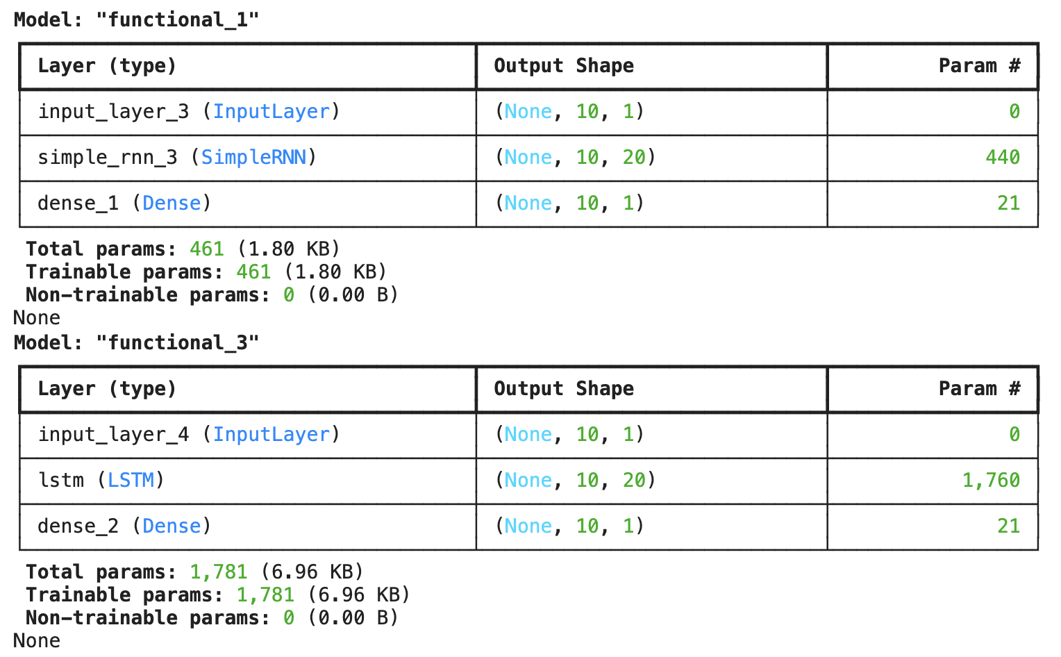
print(model_rnn.summary())
# LSTM 모델
input_lstm = Input(shape=(n_rnn, n_in))
lstm_layer = LSTM(n_mid, return_sequences=True)(input_lstm)
output_lstm = Dense(n_out, activation='linear')(lstm_layer)
model_lstm = Model(inputs=input_lstm, outputs=output_lstm)
model_lstm.compile(loss='mean_squared_error', optimizer=SGD())
print(model_lstm.summary())실행결과
2-3. 학습
import time

epochs = 500
batch_size = 8

# 일반적인 RNN
start_time = time.time()
history_rnn = model_rnn.fit(x, t, epochs = epochs, batch_size=batch_size, verbose=0)
print("일반 RNN 학습 시간 : ", time.time()-start_time)

# LSTM
start_time = time.time()
history_lstm = model_lstm.fit(x, t, epochs = epochs, batch_size=batch_size, verbose=0)
print("LSTM 학습 시간 : ", time.time()-start_time)
실행결과
일반 RNN 학습 시간 :  22.174253940582275
LSTM 학습 시간 :  23.063738346099854
LSTM의 파라미터가 더 많기 때문에 학습에 더 많은 시간이 걸린다.
2-4. 학습의 추이 관찰하기
loss_rnn = history_rnn.history['loss']
loss_lstm = history_lstm.history['loss']

plt.plot(np.arange(len(loss_rnn)), loss_rnn, label='RNN')
plt.plot(np.arange(len(loss_lstm)), loss_lstm, label='LSTM')
plt.legend()
plt.show()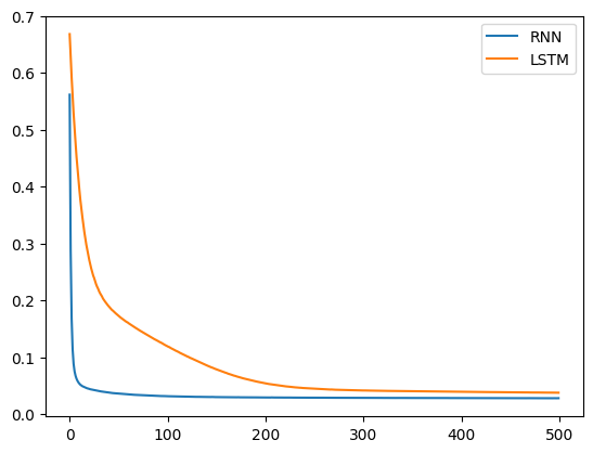
RNN과 비교했을 때, 오차가 수렴하기 위해서는 LSTM쪽이 더 많은 epoch 수가 필요했다.
2-5. 학습한 모델 사용하기
각각 모델로 sin() 함수의 다음 값을 예측한다.
predicted_rnn = x[0].reshape(-1)
predicted_lstm = x[0].reshape(-1)

for i in range(1, len(x)):
  y_rnn = model_rnn.predict(predicted_rnn[-n_rnn:].reshape(1, n_rnn, 1))
  predicted_rnn = np.append(predicted_rnn, y_rnn[0][n_rnn-1][0])

  y_lstm = model_lstm.predict(predicted_lstm[-n_rnn:].reshape(1, n_rnn, 1))
  predicted_lstm = np.append(predicted_lstm, y_lstm[0][n_rnn-1][0])

plt.plot(np.arange(len(sin_data)), sin_data, label='Training Data')
plt.plot(np.arange(len(predicted_rnn)), predicted_rnn, label='Predicted_RNN')
plt.plot(np.arange(len(predicted_lstm)), predicted_lstm, label='Predicted_LSTM')
plt.legend()
plt.show()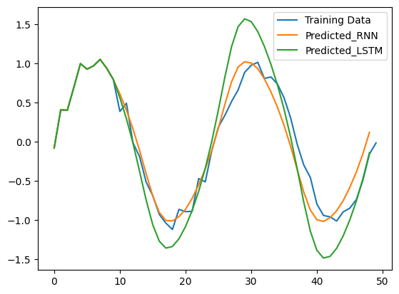
일반적인 RNN쪽이 원래의 데이터에 좀더 일치했다.
LSTM은 문맥이 중요한 자연어 처리 등의 분야에서 더 효과가 좋다.