LSA (Latent Semantic Analysis) 잠재 의미 분석

단어의 빈도수를 이용해 문장의 주제를 찾는 대신 문서의 잠재된 의미를 찾아내는 의미분석 방법
SVD 를 사용한다
토픽모델링에 자주 사용
단어-문서 행렬을 SVD로 분해하여 주요 의미 축만 남기고 불필요한 노이즈를 제거

SVD (Singular Value Decomposition, 특이값 분해)

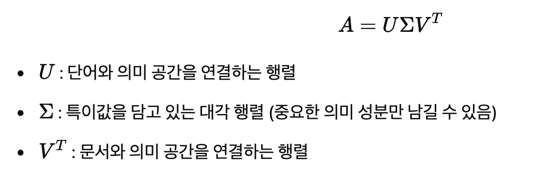
중요한 정보만 유지하고 차원 축소를 하기위해 사용된다
크기가 다른 행렬에서도 적용할 수 있다
단어와 문서 간의 관계를 더 의미 있는 공간에서 표현하는 데 활용

import numpy as np
import pandas as pd
from sklearn.decomposition import TruncatedSVD
from sklearn.feature_extraction.text import TfidfVectorizer

# 1️⃣ 샘플 문서 데이터
documents = [
    "I love deep learning and machine learning.",
    "Deep learning and AI are amazing technologies.",
    "Natural language processing is a part of AI.",
    "Machine learning is used for AI and data science.",
    "I enjoy studying AI and machine learning."
]

# 2️⃣ TF-IDF 벡터화 (단어-문서 행렬 생성)
vectorizer = TfidfVectorizer(stop_words='english')
X = vectorizer.fit_transform(documents)

# 3️⃣ SVD 적용 (LSA 수행) → 차원을 2로 줄임
n_components = 2  # 주성분 개수
svd = TruncatedSVD(n_components=n_components)
X_reduced = svd.fit_transform(X)

# 4️⃣ 결과 출력
print("🔹 원본 TF-IDF 행렬 크기:", X.shape)
print("🔹 차원 축소 후 행렬 크기:", X_reduced.shape)
print("\n🔹 변환된 문서 벡터:")
print(X_reduced)

# 5️⃣ 주성분 분석 결과 확인 (단어-주성분 관계)
terms = vectorizer.get_feature_names_out()
components_df = pd.DataFrame(svd.components_, columns=terms, index=[f"Topic {i+1}" for i in range(n_components)])
print("\n🔹 주성분(토픽)별 주요 단어:")
print(components_df)

---------------------------------------------------------------------
🔹 원본 TF-IDF 행렬 크기: (5, 15)
🔹 차원 축소 후 행렬 크기: (5, 2)

🔹 변환된 문서 벡터:
[[ 0.75238578 -0.28178464]
 [ 0.6351635  -0.07500513]
 [ 0.20911764  0.95501691]
 [ 0.63397735  0.04896327]
 [ 0.67840463  0.04259817]]

🔹 주성분(토픽)별 주요 단어:
               ai   amazing      data      deep     enjoy  language  learning  \
Topic 1  0.350064  0.186842  0.167291  0.327085  0.206008  0.061220  0.561852   
Topic 2  0.299022 -0.041325  0.024199 -0.157039  0.024228  0.523659 -0.168755   

             love   machine   natural  processing   science  studying  \
Topic 1  0.218571  0.396382  0.061220    0.061220  0.167291  0.206008   
Topic 2 -0.153321 -0.070249  0.523659    0.523659  0.024199  0.024228   

         technologies      used  
Topic 1      0.186842  0.167291  
Topic 2     -0.041325  0.024199  

문서가 2차원 벡터로 변환
topic1 : machine, learning, ai, deep 등과 관련
topic2 : natural, language, processing, studying 등과 관련

유사한 문서들을 구분 후 중요한 단어를 자동으로 그룹화

import numpy as np
import pandas as pd
import matplotlib.pyplot as plt
from sklearn.decomposition import TruncatedSVD
from sklearn.feature_extraction.text import TfidfVectorizer
from sklearn.manifold import TSNE

# 1️⃣ 샘플 문서 데이터
documents = [
    "I love deep learning and machine learning.",
    "Deep learning and AI are amazing technologies.",
    "Natural language processing is a part of AI.",
    "Machine learning is used for AI and data science.",
    "I enjoy studying AI and machine learning."
]

# 2️⃣ TF-IDF 벡터화 (단어-문서 행렬 생성)
vectorizer = TfidfVectorizer(stop_words='english')
X = vectorizer.fit_transform(documents)

# 3️⃣ LSA 적용 (SVD 기반 차원 축소, 2차원으로 변환)
n_components = 2
svd = TruncatedSVD(n_components=n_components)
X_reduced = svd.fit_transform(X)

# 4️⃣ t-SNE 추가 변환 (✅ perplexity 조정: 샘플 수(5)보다 작게 설정)
X_embedded = TSNE(n_components=2, perplexity=2, random_state=42).fit_transform(X_reduced)

# 5️⃣ 시각화 (각 문서를 2D 공간에 표현)
plt.figure(figsize=(8, 6))
plt.scatter(X_embedded[:, 0], X_embedded[:, 1], color='blue')

# 6️⃣ 각 문서에 라벨 추가
for i, doc in enumerate(documents):
    plt.annotate(f"Doc {i+1}", (X_embedded[i, 0], X_embedded[i, 1]))

plt.title("LSA embedding")
plt.xlabel("LSA Component 1")
plt.ylabel("LSA Component 2")
plt.show()

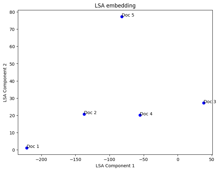
문서를 2차원 공간에 투영
비슷한 문서는 가까이에, 다른 문서는 멀리에 위치

---

LDA (Latent Dirichlet Allocation, 잠재 디리클레 할당)

토픽의 개수를 정해 모든 단어를 하나의 토픽에 할당하는 작업을 반복
각 단어가 특정 주제에서 생성될 확률을 계산하는 확률 기반 주제 모델링 기법

import numpy as np
import pandas as pd
from sklearn.feature_extraction.text import CountVectorizer
from sklearn.decomposition import LatentDirichletAllocation

# 1️⃣ 샘플 문서 데이터
documents = [
    "I love deep learning and machine learning.",
    "Deep learning and AI are amazing technologies.",
    "Natural language processing is a part of AI.",
    "Machine learning is used for AI and data science.",
    "I enjoy studying AI and machine learning."
]

# 2️⃣ 단어-문서 행렬 생성 (CountVectorizer 사용)
vectorizer = CountVectorizer(stop_words='english')
X = vectorizer.fit_transform(documents)

# 3️⃣ LDA 모델 학습 (주제 개수 2개로 설정)
n_topics = 2
lda = LatentDirichletAllocation(n_components=n_topics, random_state=42)
X_topics = lda.fit_transform(X)

# 4️⃣ 주제별 단어 출력
terms = vectorizer.get_feature_names_out()
topics_df = pd.DataFrame(lda.components_, columns=terms, index=[f"Topic {i+1}" for i in range(n_topics)])
print("\n🔹 주제별 주요 단어:")
print(topics_df)

# 5️⃣ 각 문서의 주제 비율 출력
print("\n🔹 문서별 주제 분포:")
print(pd.DataFrame(X_topics, columns=[f"Topic {i+1}" for i in range(n_topics)]))


# LDA 시각화 (lda_model 버전 사용)
pyLDAvis.enable_notebook()
vis = pyLDAvis.lda_model.prepare(lda, X, vectorizer)  # ✅ Use lda_model instead of sklearn
pyLDAvis.display(vis)
-----------------------------------------------------------------------------

🔹 주제별 주요 단어:
               ai   amazing      data      deep     enjoy  language  learning  \
Topic 1  2.601366  1.491945  0.529545  2.492414  1.491187  0.504159  5.120539   
Topic 2  2.398634  0.508055  1.470455  0.507586  0.508813  1.495841  0.879461   

             love  machine   natural  processing   science  studying  \
Topic 1  1.493296  2.84328  0.504159    0.504159  0.529545  1.491187   
Topic 2  0.506704  1.15672  1.495841    1.495841  1.470455  0.508813   

         technologies      used  
Topic 1      1.491945  0.529545  
Topic 2      0.508055  1.470455  

🔹 문서별 주제 분포:
    Topic 1   Topic 2
0  0.911026  0.088974
1  0.904009  0.095991
2  0.108849  0.891151
3  0.267629  0.732371
4  0.900698  0.099302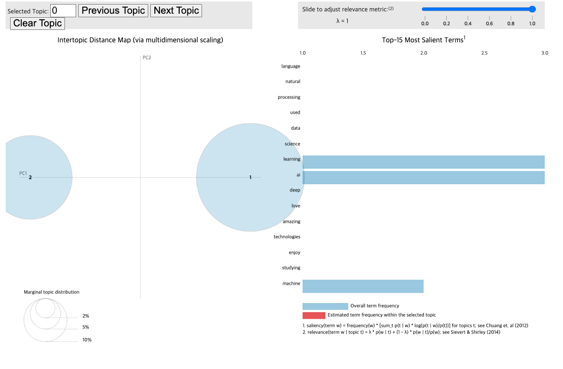

원 = 주제
원의 크기 = 주제의 중요도
원 사이의 거리 = 주제간 차이

오른쪽 = 핵심단어
λ 값 조정시 특정 주제에 대한 중요단어들을 더 볼수 있다
λ = 1 : 가장 중요한 단어만 필터링, 낮출경우 특정주제에 대한 단어 강조