🤗 소개
앞 글에서는 tractable한 score matching 목적 함수를 통해 score 기반 생성 모델의 이론적 토대를 마련했다. 그러나 해당 목적 함수는 score의 Jacobian과 trace를 포함하므로, 고차원 공간에서는 계산 비용이 크고 구현이 까다롭다는 문제 가 있다. 이번 글에서는 이러한 실용적인 한계를 어떻게 극복할 수 있는지를 살펴본다. 특히 score matching의 구조를 재해석한 Denoising Score Matching(DSM) 을 소개함으로써, 보다 효율적이고 안정적인 학습 방법으로 이어지는 동기를 제시할 예정이다. 이번 글에서는 많은 수학적 증명들이 나타나므로 꽤 긴 글이 될 것으로 예상된다.
🌦️ DSM 파헤치기
1️⃣ DSM이 태동하게 된 배경
이전 글에서 소개한 대안 목적 함수
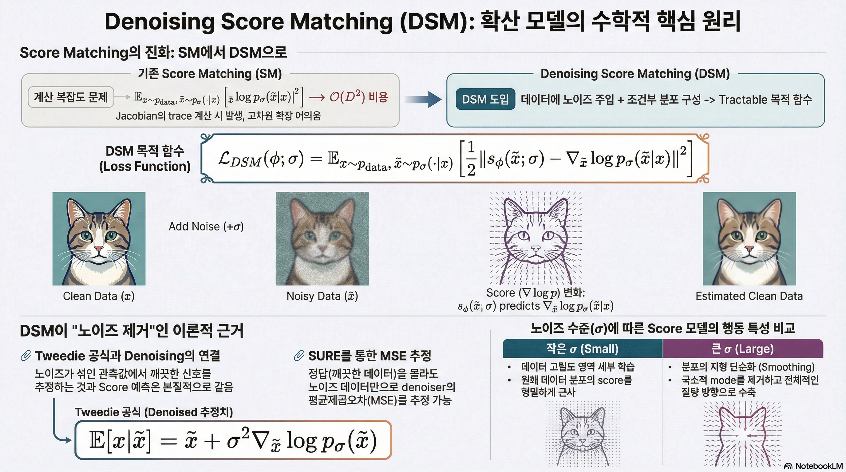
L ~ SM ( ϕ ) = E x ∼ p data [ Tr ( ∇ x s ϕ ( x ) ) + 1 2 ∥ s ϕ ( x ) ∥ 2 2 ] \tilde{\mathcal{L}}_\text{SM}(\phi)=\mathbb{E}_{\mathbf{x}\sim p_\text{data}}\left[\operatorname{Tr}(\nabla_\mathbf{x}\mathbf{s}_\phi(\mathbf{x}))+\frac{1}{2}\|\mathbf{s}_\phi(\mathbf{x})\|_2^2\right] L ~ SM ( ϕ ) = E x ∼ p data [ T r ( ∇ x s ϕ ( x ) ) + 2 1 ∥ s ϕ ( x ) ∥ 2 2 ] 는 tractable 하다는 장점이 있지만, 여전히 Jacobian의 trace Tr ( ∇ x s ϕ ( x ) ) \operatorname{Tr}(\nabla_\mathbf{x}\mathbf{s}_\phi(\mathbf{x})) T r ( ∇ x s ϕ ( x ) ) O ( D 2 ) \mathcal{O}(D^2) O ( D 2 ) 고차원 데이터로의 확장성을 제한 한다.
이 문제를 해결하기 위해 sliced score matching(Song et at., 2020b) 은 무작위 투영에 기반한 확률적 추정 을 사용하여 trace 항을 대체한다. 아래에서는 이 아이디어를 간단히 개괄한다.
🥒 Sliced Score Matching과 Hutchinson 추정기
Sliced score matching은 score matching에서의 trace 항을 무작위로 선택된 "슬라이스" 방향을 따라 계산한 방향 도함수들의 평균 으로 대체한다. 예를 들어 u ∈ R D \mathbf{u}\in\mathbb{R}^D u ∈ R D E [ u ] = 0 \mathbb{E}[\mathbf{u}]=0 E [ u ] = 0 E [ u u ⊤ ] = I \mathbb{E}[\mathbf{uu}^\top]=\mathbf{I} E [ u u ⊤ ] = I
Hutchinson 항등식 에 따르면,
Tr ( A ) = E u [ u ⊤ A u ] , E u [ ( u ⊤ s ϕ ( x ) ) 2 ] = ∥ s ϕ ( x ) ∥ 2 2 \operatorname{Tr}(\mathbf{A})=\mathbb{E}_\mathbf{u}[\mathbf{u}^\top\mathbf{Au}],\quad \mathbb{E}_\mathbf{u}[(\mathbf{u}^\top\mathbf{s}_\phi(\mathbf{x}))^2]=\|\mathbf{s}_\phi(\mathbf{x})\|_2^2 T r ( A ) = E u [ u ⊤ A u ] , E u [ ( u ⊤ s ϕ ( x ) ) 2 ] = ∥ s ϕ ( x ) ∥ 2 2 가 성립한다. 이를 이용하면 다음과 같은 정확한 형태의 목적 함수를 얻는다.
L ~ SM ( ϕ ) = E x , u [ u ⊤ ( ∇ x s ϕ ( x ) ) u + 1 2 ( u ⊤ s ϕ ( x ) ) 2 ] \tilde{\mathcal{L}}_\text{SM}(\phi)=\mathbb{E}_{\mathbf{x},\mathbf{u}}\left[\mathbf{u}^\top(\nabla_\mathbf{x}\mathbf{s}_\phi(\mathbf{x}))\mathbf{u}+\frac{1}{2}(\mathbf{u}^\top\mathbf{s}_\phi(\mathbf{x}))^2\right] L ~ SM ( ϕ ) = E x , u [ u ⊤ ( ∇ x s ϕ ( x ) ) u + 2 1 ( u ⊤ s ϕ ( x ) ) 2 ] 이 목적 함수는 큰 Jacobian이나 헤시안 행렬을 명시적으로 계산하지 않고도, 자동 미분을 이용한 Jacobian-Vector Product(JVP)와 Vector-Jacobian Produuct(VJP) 연산을 통해 효율적으로 계산 할 수 있다.
무작위 probe를 K K K O ( 1 / K ) \mathcal{O}(1/K) O ( 1 / K ) 불편향 추정기(unbiased estimator) 를 얻을 수 있으며, 방향 항 u ⊤ ( ∇ x s ϕ ) u \mathbf{u}^\top(\nabla_\mathbf{x}\mathbf{s}_\phi)\mathbf{u} u ⊤ ( ∇ x s ϕ ) u
직관적으로 보면, 이는 모델의 움직임을 무작위 방향들에서만 검사하는 것 과 같다. 투영된 score는 데이터 밀도가 더 높은 영역과 정렬되도록 유도되며, 그 결과 데이터 포인트들은 기댓값의 측면에서 정류점 들이 된다.
🧼 Sliced Score Matching에서 Denoising Score Matching으로
Sliced score matching은 Jacobian 계산을 피할 수는 있지만, 여전히 원래의 데이터 분포에 직접적으로 의존한다는 한계 를 가진다. 이로 인해 다음과 같은 취약점을 가질 수 있다. 예를 들어 이미지 데이터가 저차원 다양체(manifold) 위에 놓여 있는 경우, ∇ x log p data ( x ) \nabla_\mathbf{x}\log p_\text{data}(\mathbf{x}) ∇ x log p data ( x ) 정의되지 않거나 매우 불안정 할 수 있다.
또한, 이 방법은 관측된 데이터 지점에서만 벡터장을 제약하므로, 그 주변 영역에 대해서는 약한 제어만 을 제공한다. 추가적으로, 무작위 probe로 인한 분산 문제와 JVP/VJP 연산을 반복적으로 수행해야 하는 비용 역시 존재한다.
이번 글에서 중점적으로 다룰 보다 강력한 대안은 Denoising Score Matching(DSM; Vincent, 2011) 이다. DSM은 원리적으로 타당하면서도 확장성이 뛰어난 해결책을 제공한다.
2️⃣ DSM의 훈련
앞서 소개한 score matching 손실을 다시 살펴보자.
L SM ( ϕ ) = 1 2 E x ∼ p data ( x ) [ ∥ s ϕ ( x ) − ∇ x log p data ( x ) ∥ 2 2 ] \mathcal{L}_\text{SM}(\phi)=\frac{1}{2}\mathbb{E}_{\mathbf{x}\sim p_\text{data}(\mathbf{x})}\left[\|\mathbf{s}_\phi(\mathbf{x})-\nabla_\mathbf{x}\log p_\text{data}(\mathbf{x})\|_2^2\right] L SM ( ϕ ) = 2 1 E x ∼ p data ( x ) [ ∥ s ϕ ( x ) − ∇ x log p data ( x ) ∥ 2 2 ] 여기서 문제가 되는 부분은 intractable 한 항 ∇ x log p data ( x ) \nabla_\mathbf{x}\log p_\text{data}(\mathbf{x}) ∇ x log p data ( x )
☝🏻 조건화를 통한 해결
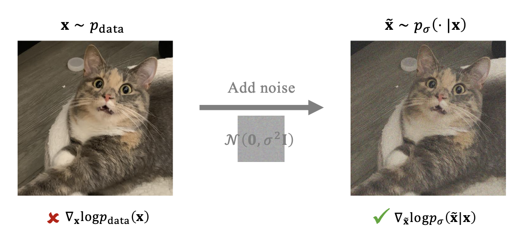
∇ x log p data ( x ) \nabla_\mathbf{x}\log p_\text{data}(\mathbf{x}) ∇ x log p data ( x ) 조건부 분포 p σ ( x ~ ∣ x ) p_\sigma(\tilde{\mathbf{x}}|\mathbf{x}) p σ ( x ~ ∣ x ) x ∼ p data \mathbf{x}\sim p_\text{data} x ∼ p data 노이즈를 주입하는 방법 을 제안했다.
신경망 s ϕ ( x ~ ; σ ) \mathbf{s}_\phi(\tilde{\mathbf{x}};\sigma) s ϕ ( x ~ ; σ ) 주변 교란 분포(marginal perturbed distribution) 를 근사하도록 학습된다.
p σ ( x ~ ) = ∫ p σ ( x ~ ∣ x ) p data ( x ) d x p_\sigma(\tilde{\mathbf{x}})=\int p_\sigma(\tilde{\mathbf{x}}|\mathbf{x})p_\text{data}(\mathbf{x})d\mathbf{x} p σ ( x ~ ) = ∫ p σ ( x ~ ∣ x ) p data ( x ) d x 이를 위해 다음 손실을 최소화한다.
L SM ( ϕ ; σ ) : = 1 2 E x ~ ∼ p σ [ ∥ s ϕ ( x ~ ; σ ) − ∇ x ~ log p σ ( x ~ ) ∥ 2 2 ] \mathcal{L}_\text{SM}(\phi;\sigma):=\frac{1}{2}\mathbb{E}_{\tilde{\mathbf{x}}\sim p_\sigma}\left[\|\mathbf{s}_\phi(\tilde{\mathbf{x}};\sigma)-\nabla_{\tilde{\mathbf{x}}}\log p_\sigma(\tilde{\mathbf{x}})\|_2^2\right] L SM ( ϕ ; σ ) : = 2 1 E x ~ ∼ p σ [ ∥ s ϕ ( x ~ ; σ ) − ∇ x ~ log p σ ( x ~ ) ∥ 2 2 ] 비록 ∇ x ~ log p σ ( x ~ ) \nabla_{\tilde{\mathbf{x}}}\log p_\sigma(\tilde{\mathbf{x}}) ∇ x ~ log p σ ( x ~ ) x ∼ p data \mathbf{x}\sim p_\text{data} x ∼ p data Denoising Score Matching(DSM) 손실을 얻을 수 있음을 보였다.
L DSM ( ϕ ; σ ) : = 1 2 E x ∼ p data x ~ ∼ p σ ( ⋅ ∣ x ) [ ∥ s ϕ ( x ~ ; σ ) − ∇ x ~ log p σ ( x ~ ∣ x ) ∥ 2 2 ] \mathcal{L}_\text{DSM}(\phi;\sigma):=\frac{1}{2}\mathbb{E}_{\mathbf{x}\sim p_\text{data}\tilde{\mathbf{x}}\sim p_\sigma(\cdot|\mathbf{x})}\left[\|\mathbf{s}_\phi(\tilde{\mathbf{x}};\sigma)-\nabla_{\tilde{\mathbf{x}}}\log p_\sigma(\tilde{\mathbf{x}}|\mathbf{x})\|_2^2\right] L DSM ( ϕ ; σ ) : = 2 1 E x ∼ p data x ~ ∼ p σ ( ⋅ ∣ x ) [ ∥ s ϕ ( x ~ ; σ ) − ∇ x ~ log p σ ( x ~ ∣ x ) ∥ 2 2 ]
위 식의 최적해 s ∗ \mathbf{s}^\ast s ∗
s ∗ ( x ~ ; σ ) = ∇ x ~ log p σ ( x ~ ) \mathbf{s}^\ast(\tilde{\mathbf{x}};\sigma)=\nabla_{\tilde{\mathbf{x}}}\log p_\sigma(\tilde{\mathbf{x}}) s ∗ ( x ~ ; σ ) = ∇ x ~ log p σ ( x ~ ) 이는 또한 L SM \mathcal{L}_\text{SM} L SM
예를 들어 p σ ( x ~ ∣ x ) p_\sigma(\tilde{\mathbf{x}}|\mathbf{x}) p σ ( x ~ ∣ x ) σ 2 \sigma^2 σ 2 p σ ( x ~ ∣ x ) = N ( x ~ ; x , σ 2 I ) p_\sigma(\tilde{\mathbf{x}}|\mathbf{x})=\mathcal{N}(\tilde{\mathbf{x}};\mathbf{x},\sigma^2\mathbf{I}) p σ ( x ~ ∣ x ) = N ( x ~ ; x , σ 2 I ) ∇ x ~ log p σ ( x ~ ∣ x ) \nabla_{\tilde{\mathbf{x}}}\log p_\sigma(\tilde{\mathbf{x}}|\mathbf{x}) ∇ x ~ log p σ ( x ~ ∣ x ) closed-form 으로 표현될 수 있다. 이로 인해 회귀의 목표가 명시적으로 주어지며 tractable하다. 또한 σ ≈ 0 \sigma\approx0 σ ≈ 0 p σ ( x ~ ) ≈ p data ( x ) p_\sigma(\tilde{\mathbf{x}})\approx p_\text{data}(\mathbf{x}) p σ ( x ~ ) ≈ p data ( x )
s ∗ ( x ~ ; σ ) = ∇ x ~ log p σ ( x ~ ) ≈ ∇ x log p data ( x ) \mathbf{s}^\ast(\tilde{\mathbf{x}};\sigma)=\nabla_{\tilde{\mathbf{x}}}\log p_\sigma(\tilde{\mathbf{x}})\approx\nabla_\mathbf{x}\log p_\text{data}(\mathbf{x}) s ∗ ( x ~ ; σ ) = ∇ x ~ log p σ ( x ~ ) ≈ ∇ x log p data ( x ) 가 성립한다. 이는 학습된 score가 원래 데이터 분포의 score를 근사하게 됨 을 의미하며, 이를 생성 과정에 활용할 수 있음을 보여준다.
이러한 논의를 바탕으로 L SM \mathcal{L}_\text{SM} L SM L DSM \mathcal{L}_\text{DSM} L DSM
정리 3.3.1 – L SM \mathcal{L}_\text{SM} L SM L DSM \mathcal{L}_\text{DSM} L DSM σ > 0 \sigma>0 σ > 0
L SM ( ϕ ; σ ) = L DSM ( ϕ ; σ ) + C \mathcal{L}_\text{SM}(\phi;\sigma)=\mathcal{L}_\text{DSM}(\phi;\sigma)+C L SM ( ϕ ; σ ) = L DSM ( ϕ ; σ ) + C 여기서 C C C ϕ \phi ϕ s ∗ ( ⋅ ; σ ) \mathbf{s}^\ast(\cdot;\sigma) s ∗ ( ⋅ ; σ )
s ∗ ( ⋅ ; σ ) = ∇ x ~ log p σ ( x ~ ) , for almost every x ~ \mathbf{s}^\ast(\cdot;\sigma)=\nabla_{\tilde{\mathbf{x}}}\log p_\sigma(\tilde{\mathbf{x}}),\quad\text{for almost every}~\tilde{\mathbf{x}} s ∗ ( ⋅ ; σ ) = ∇ x ~ log p σ ( x ~ ) , for almost every x ~
💡 정리 3.3.1에서 등가성에 대한 증명
L SM ( ϕ ; σ ) \mathcal{L}_\text{SM}(\phi;\sigma) L SM ( ϕ ; σ ) L DSM ( ϕ ; σ ) \mathcal{L}_\text{DSM}(\phi;\sigma) L DSM ( ϕ ; σ )
L SM ( ϕ ; σ ) = 1 2 E x ~ ∼ p σ ( x ~ ) [ ∥ s ϕ ( x ~ ; σ ) ∥ 2 2 − 2 s ϕ ( x ~ ; σ ) ⊤ ∇ x ~ log p σ ( x ~ ) + ∥ ∇ x ~ log p σ ( x ~ ) ∥ 2 2 ] L DSM ( ϕ ; σ ) = 1 2 E p data ( x ) p σ ( x ~ ∣ x ) [ ∥ s ϕ ( x ~ ; σ ) ∥ 2 2 − 2 s ϕ ( x ~ ; σ ) ⊤ ∇ x ~ log p σ ( x ~ ∣ x ) + ∥ ∇ x ~ log p σ ( x ~ ∣ x ) ∥ 2 2 ] \small \begin{aligned} \mathcal{L}_\text{SM}(\phi;\sigma)&=\frac{1}{2}\mathbb{E}_{\tilde{\mathbf{x}}\sim p_\sigma(\tilde{\mathbf{x}})}\left[\|\mathbf{s}_\phi(\tilde{\mathbf{x}};\sigma)\|_2^2-2\mathbf{s}_\phi(\tilde{\mathbf{x}};\sigma)^\top\nabla_{\tilde{\mathbf{x}}}\log p_\sigma(\tilde{\mathbf{x}})+\|\nabla_{\tilde{\mathbf{x}}}\log p_\sigma(\tilde{\mathbf{x}})\|_2^2\right] \\ \mathcal{L}_\text{DSM}(\phi;\sigma)&=\frac{1}{2}\mathbb{E}_{p_\text{data}(\mathbf{x})p_\sigma(\tilde{\mathbf{x}}|\mathbf{x})}\left[\|\mathbf{s}_\phi(\tilde{\mathbf{x}};\sigma)\|_2^2-2\mathbf{s}_\phi(\tilde{\mathbf{x}};\sigma)^\top\nabla_{\tilde{\mathbf{x}}}\log p_\sigma(\tilde{\mathbf{x}}|\mathbf{x})+\|\nabla_{\tilde{\mathbf{x}}}\log p_\sigma(\tilde{\mathbf{x}}|\mathbf{x})\|_2^2\right] \\ \end{aligned} L SM ( ϕ ; σ ) L DSM ( ϕ ; σ ) = 2 1 E x ~ ∼ p σ ( x ~ ) [ ∥ s ϕ ( x ~ ; σ ) ∥ 2 2 − 2 s ϕ ( x ~ ; σ ) ⊤ ∇ x ~ log p σ ( x ~ ) + ∥ ∇ x ~ log p σ ( x ~ ) ∥ 2 2 ] = 2 1 E p data ( x ) p σ ( x ~ ∣ x ) [ ∥ s ϕ ( x ~ ; σ ) ∥ 2 2 − 2 s ϕ ( x ~ ; σ ) ⊤ ∇ x ~ log p σ ( x ~ ∣ x ) + ∥ ∇ x ~ log p σ ( x ~ ∣ x ) ∥ 2 2 ] 이 두 손실에 대해 뺄셈을 적용하면,
L SM ( ϕ ; σ ) − L DSM ( ϕ ; σ ) = 1 2 ( E x ~ ∼ p σ ( x ~ ) ∥ s ϕ ( x ~ ; σ ) ∥ 2 2 − E p data ( x ) p σ ( x ~ ∣ x ) ∥ s ϕ ( x ~ ; σ ) ∥ 2 2 ) − ( E x ~ ∼ p σ ( x ~ ) [ s ϕ ( x ~ ; σ ) ⊤ ∇ x ~ log p σ ( x ~ ) ] − E p data ( x ) p σ ( x ~ ∣ x ) [ s ϕ ( x ~ ; x ) ⊤ ∇ x ~ log p σ ( x ~ ∣ x ) ] ) + 1 2 ( E x ~ ∼ p σ ( x ~ ) ∥ ∇ x ~ log p σ ( x ~ ) ∥ 2 2 − E p data ( x ) p σ ( x ~ ∣ x ) ∥ ∇ x ~ log p σ ( x ~ ∣ x ) ∥ 2 2 ) \begin{aligned} &\quad\mathcal{L}_\text{SM}(\phi;\sigma)-\mathcal{L}_\text{DSM}(\phi;\sigma) \\ &=\frac{1}{2}\bigg(\mathbb{E}_{\tilde{\mathbf{x}}\sim p_\sigma(\tilde{\mathbf{x}})}\|\mathbf{s}_\phi(\tilde{\mathbf{x}};\sigma)\|_2^2-\mathbb{E}_{p_\text{data}(\mathbf{x})p_\sigma(\tilde{\mathbf{x}}|\mathbf{x})}\|\mathbf{s}_\phi(\tilde{\mathbf{x}};\sigma)\|_2^2\bigg)\\ &\small\quad-\bigg(\mathbb{E}_{\tilde{\mathbf{x}}\sim p_\sigma(\tilde{\mathbf{x}})}\left[\mathbf{s}_\phi(\tilde{\mathbf{x}};\sigma)^\top\nabla_{\tilde{\mathbf{x}}}\log p_\sigma(\tilde{\mathbf{x}})\right]-\mathbb{E}_{p_\text{data}(\mathbf{x})p_\sigma(\tilde{\mathbf{x}}|\mathbf{x})}\left[\mathbf{s}_\phi(\tilde{\mathbf{x}};\mathbf{x})^\top\nabla_{\tilde{\mathbf{x}}}\log p_\sigma(\tilde{\mathbf{x}}|\mathbf{x})\right]\bigg) \\ &\quad+\frac{1}{2}\bigg(\mathbb{E}_{\tilde{\mathbf{x}}\sim p_\sigma(\tilde{\mathbf{x}})}\|\nabla_{\tilde{\mathbf{x}}}\log p_\sigma(\tilde{\mathbf{x}})\|_2^2-\mathbb{E}_{p_\text{data}(\mathbf{x})p_\sigma(\tilde{\mathbf{x}}|\mathbf{x})}\|\nabla_{\tilde{\mathbf{x}}}\log p_\sigma(\tilde{\mathbf{x}}|\mathbf{x})\|_2^2\bigg) \\ \end{aligned} L SM ( ϕ ; σ ) − L DSM ( ϕ ; σ ) = 2 1 ( E x ~ ∼ p σ ( x ~ ) ∥ s ϕ ( x ~ ; σ ) ∥ 2 2 − E p data ( x ) p σ ( x ~ ∣ x ) ∥ s ϕ ( x ~ ; σ ) ∥ 2 2 ) − ( E x ~ ∼ p σ ( x ~ ) [ s ϕ ( x ~ ; σ ) ⊤ ∇ x ~ log p σ ( x ~ ) ] − E p data ( x ) p σ ( x ~ ∣ x ) [ s ϕ ( x ~ ; x ) ⊤ ∇ x ~ log p σ ( x ~ ∣ x ) ] ) + 2 1 ( E x ~ ∼ p σ ( x ~ ) ∥ ∇ x ~ log p σ ( x ~ ) ∥ 2 2 − E p data ( x ) p σ ( x ~ ∣ x ) ∥ ∇ x ~ log p σ ( x ~ ∣ x ) ∥ 2 2 ) 이제 이 식을 한번에 한 항씩 살펴보자. 우선 첫번째 항부터 보자면, p σ ( x ~ ) = ∫ p σ ( x ~ ∣ x ) p data ( x ) d x p_\sigma(\tilde{\mathbf{x}})=\int p_\sigma(\tilde{\mathbf{x}}|\mathbf{x})p_\text{data}(\mathbf{x})d\mathbf{x} p σ ( x ~ ) = ∫ p σ ( x ~ ∣ x ) p data ( x ) d x
E x ~ ∼ p σ ( x ~ ) ∥ s ϕ ( x ~ ; σ ) ∥ 2 2 = ∫ ( ∫ p σ ( x ~ ∣ x ) p data ( x ) d x ) ∥ s ϕ ( x ~ ; σ ) ∥ 2 2 d x ~ = ∫ p data ( x ) ∫ p σ ( x ~ ∣ x ) ∥ s ϕ ( x ~ ; σ ) ∥ 2 2 d x ~ d x = E p data ( x ) p σ ( x ~ ∣ x ) ∥ s ϕ ( x ~ ; σ ) ∥ 2 2 \begin{aligned} \mathbb{E}_{\tilde{\mathbf{x}}\sim p_\sigma(\tilde{\mathbf{x}})}\|\mathbf{s}_\phi(\tilde{\mathbf{x}};\sigma)\|_2^2&=\int\bigg(\int p_\sigma(\tilde{\mathbf{x}}|\mathbf{x})p_\text{data}(\mathbf{x})d\mathbf{x}\bigg)\|\mathbf{s}_\phi(\tilde{\mathbf{x}};\sigma)\|_2^2~d\tilde{\mathbf{x}} \\ &=\int p_\text{data}(\mathbf{x})\int p_\sigma(\tilde{\mathbf{x}}|\mathbf{x})\|\mathbf{s}_\phi(\tilde{\mathbf{x}};\sigma)\|_2^2~d\tilde{\mathbf{x}}d\mathbf{x} \\ &=\mathbb{E}_{p_\text{data}(\mathbf{x})p_\sigma(\tilde{\mathbf{x}}|\mathbf{x})}\|\mathbf{s}_\phi(\tilde{\mathbf{x}};\sigma)\|_2^2 \\ \end{aligned} E x ~ ∼ p σ ( x ~ ) ∥ s ϕ ( x ~ ; σ ) ∥ 2 2 = ∫ ( ∫ p σ ( x ~ ∣ x ) p data ( x ) d x ) ∥ s ϕ ( x ~ ; σ ) ∥ 2 2 d x ~ = ∫ p data ( x ) ∫ p σ ( x ~ ∣ x ) ∥ s ϕ ( x ~ ; σ ) ∥ 2 2 d x ~ d x = E p data ( x ) p σ ( x ~ ∣ x ) ∥ s ϕ ( x ~ ; σ ) ∥ 2 2 즉, 첫 번째 항은 0 0 0
E x ~ ∼ p σ ( x ~ ) [ s ϕ ( x ~ ; σ ) ⊤ ∇ x ~ log p σ ( x ~ ) ] = ∫ p σ ( x ~ ) s ϕ ( x ~ ; σ ) ⊤ ( ∇ x ~ p σ ( x ~ ) p σ ( x ~ ) ) d x ~ = ∫ s ϕ ( x ~ ; σ ) ⊤ ∇ x ~ ∫ p σ ( x ~ ∣ x ) p data ( x ) d x d x ~ = ∬ s ϕ ( x ~ ; σ ) ⊤ ∇ x ~ p σ ( x ~ ∣ x ) p data ( x ) d x ~ d x = E p data ( x ) p σ ( x ~ ∣ x ) [ s ϕ ( x ~ ; σ ) ⊤ ∇ x ~ log p σ ( x ~ ∣ x ) ] \begin{aligned} \mathbb{E}_{\tilde{\mathbf{x}}\sim p_\sigma(\tilde{\mathbf{x}})}\left[\mathbf{s}_\phi(\tilde{\mathbf{x}};\sigma)^\top\nabla_{\tilde{\mathbf{x}}}\log p_\sigma(\tilde{\mathbf{x}})\right]&=\int p_\sigma(\tilde{\mathbf{x}})\mathbf{s}_\phi(\tilde{\mathbf{x}};\sigma)^\top\left(\frac{\nabla_{\tilde{\mathbf{x}}}p_\sigma(\tilde{\mathbf{x}})}{p_\sigma(\tilde{\mathbf{x}})}\right)d\tilde{\mathbf{x}} \\ &=\int\mathbf{s}_\phi(\tilde{\mathbf{x}};\sigma)^\top\nabla_{\tilde{\mathbf{x}}}\int p_\sigma(\tilde{\mathbf{x}}|\mathbf{x})p_\text{data}(\mathbf{x})~d\mathbf{x}d\tilde{\mathbf{x}} \\ &=\iint\mathbf{s}_\phi(\tilde{\mathbf{x}};\sigma)^\top\nabla_{\tilde{\mathbf{x}}}p_\sigma(\tilde{\mathbf{x}}|\mathbf{x})p_\text{data}(\mathbf{x})~d\tilde{\mathbf{x}}d\mathbf{x} \\ &=\mathbb{E}_{p_\text{data}(\mathbf{x})p_\sigma(\tilde{\mathbf{x}}|\mathbf{x})}\left[\mathbf{s}_\phi(\tilde{\mathbf{x}};\sigma)^\top\nabla_{\tilde{\mathbf{x}}}\log p_\sigma(\tilde{\mathbf{x}}|\mathbf{x})\right] \\ \end{aligned} E x ~ ∼ p σ ( x ~ ) [ s ϕ ( x ~ ; σ ) ⊤ ∇ x ~ log p σ ( x ~ ) ] = ∫ p σ ( x ~ ) s ϕ ( x ~ ; σ ) ⊤ ( p σ ( x ~ ) ∇ x ~ p σ ( x ~ ) ) d x ~ = ∫ s ϕ ( x ~ ; σ ) ⊤ ∇ x ~ ∫ p σ ( x ~ ∣ x ) p data ( x ) d x d x ~ = ∬ s ϕ ( x ~ ; σ ) ⊤ ∇ x ~ p σ ( x ~ ∣ x ) p data ( x ) d x ~ d x = E p data ( x ) p σ ( x ~ ∣ x ) [ s ϕ ( x ~ ; σ ) ⊤ ∇ x ~ log p σ ( x ~ ∣ x ) ] 마찬가지로 0 0 0
C : = 1 2 ( E x ~ ∼ p σ ( x ~ ) ∥ ∇ x ~ log p σ ( x ~ ) ∥ 2 2 − E p data ( x ) p σ ( x ~ ∣ x ) ∥ ∇ x ~ log p σ ( x ~ ∣ x ) ∥ 2 2 ) C:=\frac{1}{2}\bigg(\mathbb{E}_{\tilde{\mathbf{x}}\sim p_\sigma(\tilde{\mathbf{x}})}\|\nabla_{\tilde{\mathbf{x}}}\log p_\sigma(\tilde{\mathbf{x}})\|_2^2-\mathbb{E}_{p_\text{data}(\mathbf{x})p_\sigma(\tilde{\mathbf{x}}|\mathbf{x})}\|\nabla_{\tilde{\mathbf{x}}}\log p_\sigma(\tilde{\mathbf{x}}|\mathbf{x})\|_2^2\bigg) C : = 2 1 ( E x ~ ∼ p σ ( x ~ ) ∥ ∇ x ~ log p σ ( x ~ ) ∥ 2 2 − E p data ( x ) p σ ( x ~ ∣ x ) ∥ ∇ x ~ log p σ ( x ~ ∣ x ) ∥ 2 2 ) 하지만 이는 ϕ \phi ϕ
arg min ϕ L SM ( ϕ ; σ ) = arg min ϕ L DSM ( ϕ ; σ ) \boxed{ \argmin_\phi\mathcal{L}_\text{SM}(\phi;\sigma)=\argmin_\phi\mathcal{L}_\text{DSM}(\phi;\sigma) } ϕ a r g m i n L SM ( ϕ ; σ ) = ϕ a r g m i n L DSM ( ϕ ; σ ) 이므로, 두 손실은 본질적으로 동등함을 증명할 수 있다. ■ _\blacksquare ■
🪄 정리 3.3.1에서 SM과 DSM의 최소해 유도
최소해 s ∗ \mathbf{s}^\ast s ∗ t t t
J ( t , ϕ ) : = E x 0 ∼ p data E x t ∼ p t ( ⋅ ∣ x 0 ) [ ∥ s ϕ ( x t , t ) − ∇ x t log p t ( x t ∣ x 0 ) ∥ 2 2 ] \mathcal{J}(t,\phi):=\mathbb{E}_{\mathbf{x}_0\sim p_\text{data}}\mathbb{E}_{\mathbf{x}_t\sim p_t(\cdot|\mathbf{x}_0)}\left[\|\mathbf{s}_\phi(\mathbf{x}_t,t)-\nabla_{\mathbf{x}_t}\log p_t(\mathbf{x}_t|\mathbf{x}_0)\|_2^2\right] J ( t , ϕ ) : = E x 0 ∼ p data E x t ∼ p t ( ⋅ ∣ x 0 ) [ ∥ s ϕ ( x t , t ) − ∇ x t log p t ( x t ∣ x 0 ) ∥ 2 2 ] 이 기댓값을 최소화하기 위해서는 각 x t \mathbf{x}_t x t s ϕ ( x t , t ) \mathbf{s}_\phi(\mathbf{x}_t,t) s ϕ ( x t , t ) X 0 X_0 X 0 X t X_t X t
J ( t , ϕ ) = ∬ p data ( x 0 ) p t ( x t ∣ x 0 ) ∥ s ϕ ( x t , t ) − ∇ x t log p t ( x t ∣ x 0 ) ∥ 2 2 d x 0 d x t \mathcal{J}(t,\phi)=\iint p_\text{data}(\mathbf{x}_0)p_t(\mathbf{x}_t|\mathbf{x}_0)\|\mathbf{s}_\phi(\mathbf{x}_t, t)-\nabla_{\mathbf{x}_t}\log p_t(\mathbf{x}_t|\mathbf{x}_0)\|_2^2~d\mathbf{x}_0d\mathbf{x}_t J ( t , ϕ ) = ∬ p data ( x 0 ) p t ( x t ∣ x 0 ) ∥ s ϕ ( x t , t ) − ∇ x t log p t ( x t ∣ x 0 ) ∥ 2 2 d x 0 d x t 고정된 x t \mathbf{x}_t x t
∫ p ( x 0 ∣ X t = x t ) p t ( x t ) ∥ s ϕ ( x t , t ) − ∇ x t log p t ( x t ∣ x 0 ) ∥ 2 2 d x 0 \int p(\mathbf{x}_0|X_t=\mathbf{x}_t)p_t(\mathbf{x}_t)\|\mathbf{s}_\phi(\mathbf{x}_t, t)-\nabla_{\mathbf{x}_t}\log p_t(\mathbf{x}_t|\mathbf{x}_0)\|_2^2~d\mathbf{x}_0 ∫ p ( x 0 ∣ X t = x t ) p t ( x t ) ∥ s ϕ ( x t , t ) − ∇ x t log p t ( x t ∣ x 0 ) ∥ 2 2 d x 0 p t ( x t ) p_t(\mathbf{x}_t) p t ( x t ) s ϕ ( x t , t ) \mathbf{s}_\phi(\mathbf{x}_t,t) s ϕ ( x t , t )
∫ p ( x 0 ∣ X t = x t ) ∥ s ϕ ( x t , t ) − ∇ x t log p t ( x t ∣ x 0 ) ∥ 2 2 d x 0 \int p(\mathbf{x}_0|X_t=\mathbf{x}_t)\|\mathbf{s}_\phi(\mathbf{x}_t, t)-\nabla_{\mathbf{x}_t}\log p_t(\mathbf{x}_t|\mathbf{x}_0)\|_2^2~d\mathbf{x}_0 ∫ p ( x 0 ∣ X t = x t ) ∥ s ϕ ( x t , t ) − ∇ x t log p t ( x t ∣ x 0 ) ∥ 2 2 d x 0 이는 s ϕ ( x t , t ) \mathbf{s}_\phi(\mathbf{x}_t,t) s ϕ ( x t , t )
s ∗ ( x t , t ) = E x 0 ∼ p ( X 0 ∣ X t = x t ) [ ∇ x t log p t ( x t ∣ X 0 ) ] \mathbf{s}^\ast(\mathbf{x}_t,t)=\mathbb{E}_{\mathbf{x}_0\sim p(X_0|X_t=\mathbf{x}_t)}\left[\nabla_{\mathbf{x}_t}\log p_t(\mathbf{x}_t|X_0)\right] s ∗ ( x t , t ) = E x 0 ∼ p ( X 0 ∣ X t = x t ) [ ∇ x t log p t ( x t ∣ X 0 ) ] 이제 이것이 ∇ x t log p t ( x t ) \nabla_{\mathbf{x}_t}\log p_t(\mathbf{x}_t) ∇ x t log p t ( x t )
p t ( x t ) = ∫ p t ( x t ∣ x 0 ) p data ( x 0 ) d x 0 p_t(\mathbf{x}_t)=\int p_t(\mathbf{x}_t|\mathbf{x}_0)p_\text{data}(\mathbf{x}_0)~d\mathbf{x}_0 p t ( x t ) = ∫ p t ( x t ∣ x 0 ) p data ( x 0 ) d x 0 여기에 로그를 취한 뒤 x t \mathbf{x}_t x t
∇ x t log p t ( x t ) = ∇ x t p t ( x t ) p t ( x t ) = ∇ x t ∫ p t ( x t ∣ x 0 ) p data ( x 0 ) d x 0 ∫ p t ( x t ∣ x 0 ) p data ( x 0 ) d x 0 \nabla_{\mathbf{x}_t}\log p_t(\mathbf{x}_t)=\frac{\nabla_{\mathbf{x}_t}p_t(\mathbf{x}_t)}{p_t(\mathbf{x}_t)}=\frac{\nabla_{\mathbf{x}_t}\int p_t(\mathbf{x}_t|\mathbf{x}_0)p_\text{data}(\mathbf{x}_0)~d\mathbf{x}_0}{\int p_t(\mathbf{x}_t|\mathbf{x}_0)p_\text{data}(\mathbf{x}_0)~d\mathbf{x}_0} ∇ x t log p t ( x t ) = p t ( x t ) ∇ x t p t ( x t ) = ∫ p t ( x t ∣ x 0 ) p data ( x 0 ) d x 0 ∇ x t ∫ p t ( x t ∣ x 0 ) p data ( x 0 ) d x 0 적절한 정칙성 조건 하에서는 기울기 연산과 적분을 교환할 수 있으므로,
∇ x t log p t ( x t ) = ∫ ∇ x t p t ( x t ∣ x 0 ) p data ( x 0 ) d x 0 ∫ p t ( x t ∣ x 0 ) p data ( x 0 ) d x 0 \nabla_{\mathbf{x}_t}\log p_t(\mathbf{x}_t)=\frac{\int\nabla_{\mathbf{x}_t} p_t(\mathbf{x}_t|\mathbf{x}_0)p_\text{data}(\mathbf{x}_0)~d\mathbf{x}_0}{\int p_t(\mathbf{x}_t|\mathbf{x}_0)p_\text{data}(\mathbf{x}_0)~d\mathbf{x}_0} ∇ x t log p t ( x t ) = ∫ p t ( x t ∣ x 0 ) p data ( x 0 ) d x 0 ∫ ∇ x t p t ( x t ∣ x 0 ) p data ( x 0 ) d x 0 이제 s ∗ ( x t , t ) \mathbf{s}^\ast(\mathbf{x}_t,t) s ∗ ( x t , t )
s ∗ ( x t , t ) = ∫ p ( x 0 ∣ x t ) ∇ x t log p t ( x t ∣ x 0 ) d x 0 \mathbf{s}^\ast(\mathbf{x}_t,t)=\int p(\mathbf{x}_0|\mathbf{x}_t)\nabla_{\mathbf{x}_t}\log p_t(\mathbf{x}_t|\mathbf{x}_0)~d\mathbf{x}_0 s ∗ ( x t , t ) = ∫ p ( x 0 ∣ x t ) ∇ x t log p t ( x t ∣ x 0 ) d x 0 여기에도 위에서와 마찬가지로 Bayes'rule과 marginal probability의 정의를 적용하면 다음과 같다.
s ∗ ( x t , t ) = ∫ p t ( x t ∣ x 0 ) p data ( x 0 ) p t ( x t ) ∇ x t log p t ( x t ∣ x 0 ) d x 0 = ∫ p t ( x t ∣ x 0 ) p data ( x 0 ) p t ( x t ) ⋅ ∇ x t p t ( x t ∣ x 0 ) p t ( x t ∣ x 0 ) d x 0 = 1 p t ( x t ) ∫ ∇ x t p t ( x t ∣ x 0 ) p data ( x 0 ) d x 0 = ∫ ∇ x t p t ( x t ∣ x 0 ) p data ( x 0 ) d x 0 ∫ p t ( x t ∣ x 0 ) p data ( x 0 ) d x 0 \begin{aligned} \mathbf{s}^\ast(\mathbf{x}_t,t)&=\int\frac{p_t(\mathbf{x}_t|\mathbf{x}_0)p_\text{data}(\mathbf{x}_0)}{p_t(\mathbf{x}_t)}\nabla_{\mathbf{x}_t}\log p_t(\mathbf{x}_t|\mathbf{x}_0)~d\mathbf{x}_0 \\ &=\int\frac{p_t(\mathbf{x}_t|\mathbf{x}_0)p_\text{data}(\mathbf{x}_0)}{p_t(\mathbf{x}_t)}\cdot\frac{\nabla_{\mathbf{x}_t}p_t(\mathbf{x}_t|\mathbf{x}_0)}{p_t(\mathbf{x}_t|\mathbf{x}_0)}~d\mathbf{x}_0 \\ &=\frac{1}{p_t(\mathbf{x}_t)}\int\nabla_{\mathbf{x}_t}p_t(\mathbf{x}_t|\mathbf{x}_0)p_\text{data}(\mathbf{x}_0)~d\mathbf{x}_0 \\ &=\frac{\int\nabla_{\mathbf{x}_t} p_t(\mathbf{x}_t|\mathbf{x}_0)p_\text{data}(\mathbf{x}_0)~d\mathbf{x}_0}{\int p_t(\mathbf{x}_t|\mathbf{x}_0)p_\text{data}(\mathbf{x}_0)~d\mathbf{x}_0} \\ \end{aligned} s ∗ ( x t , t ) = ∫ p t ( x t ) p t ( x t ∣ x 0 ) p data ( x 0 ) ∇ x t log p t ( x t ∣ x 0 ) d x 0 = ∫ p t ( x t ) p t ( x t ∣ x 0 ) p data ( x 0 ) ⋅ p t ( x t ∣ x 0 ) ∇ x t p t ( x t ∣ x 0 ) d x 0 = p t ( x t ) 1 ∫ ∇ x t p t ( x t ∣ x 0 ) p data ( x 0 ) d x 0 = ∫ p t ( x t ∣ x 0 ) p data ( x 0 ) d x 0 ∫ ∇ x t p t ( x t ∣ x 0 ) p data ( x 0 ) d x 0 따라서 다음과 같이 SM과 DSM 공통의 최소해 s ∗ \mathbf{s}^\ast s ∗
s ∗ ( x t , t ) = E x 0 ∼ p ( X 0 ∣ X t = x t ) [ ∇ x t log p t ( x t ∣ X 0 ) ] = ∇ x t log p t ( x t ) ■ \boxed{ \mathbf{s}^\ast(\mathbf{x}_t,t)=\mathbb{E}_{\mathbf{x}_0\sim p(X_0|X_t=\mathbf{x}_t)}\left[\nabla_{\mathbf{x}_t}\log p_t(\mathbf{x}_t|X_0)\right]=\nabla_{\mathbf{x}_t}\log p_t(\mathbf{x}_t)}\quad_\blacksquare s ∗ ( x t , t ) = E x 0 ∼ p ( X 0 ∣ X t = x t ) [ ∇ x t log p t ( x t ∣ X 0 ) ] = ∇ x t log p t ( x t ) ■ 마치 이전에 소개한 DDPM에서처럼, 정리 3.3.1은 조건화로부터 다음과 같은 통찰을 얻을 수 있게 해준다.
통찰 3.3.1 – 조건화 기법 정리 2.2.1 ). 이 경우 데이터 포인트 x \mathbf{x} x
🌟 특수한 경우: 가산적 Gaussian 노이즈
이제 각 데이터 포인트 x ∼ p data \mathbf{x}\sim p_\text{data} x ∼ p data σ 2 \sigma^2 σ 2 N ( 0 , σ 2 I ) \mathcal{N}(\mathbf{0},\sigma^2\mathbf{I}) N ( 0 , σ 2 I )
ϵ ∼ N ( 0 , I ) , x ~ = x + σ ϵ \epsilon\sim\mathcal{N}(\mathbf{0},\mathbf{I}),\quad\tilde{\mathbf{x}}=\mathbf{x}+\sigma\epsilon ϵ ∼ N ( 0 , I ) , x ~ = x + σ ϵ 로 설정하면, 노이즈가 섞인 데이터 x ~ \tilde{\mathbf{x}} x ~
p σ ( x ~ ∣ x ) = N ( x ~ ; x , σ 2 I ) p_\sigma(\tilde{\mathbf{x}}|\mathbf{x})=\mathcal{N}(\tilde{\mathbf{x}};\mathbf{x},\sigma^2\mathbf{I}) p σ ( x ~ ∣ x ) = N ( x ~ ; x , σ 2 I ) 이 설정에서 조건부 score는 해석적으로 다음과 같이 주어진다.
∇ x ~ log p σ ( x ~ ∣ x ) = x − x ~ σ 2 \nabla_{\tilde{\mathbf{x}}}\log p_\sigma(\tilde{\mathbf{x}}|\mathbf{x})=\frac{\mathbf{x}-\tilde{\mathbf{x}}}{\sigma^2} ∇ x ~ log p σ ( x ~ ∣ x ) = σ 2 x − x ~ 따라서 DSM 손실은 다음과 같이 단순화된다.
L DSM ( ϕ ; σ ) = 1 2 E x , x ~ ∣ x [ ∥ s ϕ ( x ~ ; σ ) − x − x ~ σ 2 ∥ 2 2 ] = 1 2 E x , ϵ [ ∥ s ϕ ( x + σ ϵ ; σ ) + ϵ σ ∥ 2 2 ] \boxed{ \begin{aligned} \mathcal{L}_\text{DSM}(\phi;\sigma)&=\frac{1}{2}\mathbb{E}_{\mathbf{x},\tilde{\mathbf{x}}|\mathbf{x}}\bigg[\bigg\Vert \mathbf{s}_\phi(\tilde{\mathbf{x}};\sigma)-\frac{\mathbf{x}-\tilde{\mathbf{x}}}{\sigma^2}\bigg\Vert_2^2\bigg] \\ &=\frac{1}{2}\mathbb{E}_{\mathbf{x},\epsilon}\bigg[\bigg\Vert \mathbf{s}_\phi(\mathbf{x}+\sigma\epsilon;\sigma)+\frac{\epsilon}{\sigma}\bigg\Vert_2^2\bigg] \\ \end{aligned} } L DSM ( ϕ ; σ ) = 2 1 E x , x ~ ∣ x [ ∥ ∥ ∥ ∥ ∥ s ϕ ( x ~ ; σ ) − σ 2 x − x ~ ∥ ∥ ∥ ∥ ∥ 2 2 ] = 2 1 E x , ϵ [ ∥ ∥ ∥ ∥ ∥ s ϕ ( x + σ ϵ ; σ ) + σ ϵ ∥ ∥ ∥ ∥ ∥ 2 2 ] 여기서 ϵ ∼ N ( 0 , I ) \epsilon\sim\mathcal{N}(\mathbf{0},\mathbf{I}) ϵ ∼ N ( 0 , I ) score-based diffusion 모델의 핵심 을 이룬다.
노이즈 수준 σ \sigma σ p σ = p data ∗ N ( 0 , σ 2 I ) p_\sigma=p_\text{data}\ast\mathcal{N}(\mathbf{0},\sigma^2\mathbf{I}) p σ = p data ∗ N ( 0 , σ 2 I ) 거의 동일한 고밀도 영역과 score를 갖게 된다.
∇ x ~ log p σ ( x ~ ) ≈ ∇ x log p data ( x ) \nabla_{\tilde{\mathbf{x}}}\log p_\sigma(\tilde{\mathbf{x}})\approx\nabla_\mathbf{x}\log p_\text{data}(\mathbf{x}) ∇ x ~ log p σ ( x ~ ) ≈ ∇ x log p data ( x ) 따라서 노이즈가 섞인 score 방향 ∇ x ~ log p σ \nabla_{\tilde{\mathbf{x}}}\log p_\sigma ∇ x ~ log p σ 거의 동일한 영역으로 이동 하게 된다. 이는 앞서 요약한 score matching의 직관과 유사하다.
반대로 σ \sigma σ 과도하게 단순화 한다. 즉, p σ p_\sigma p σ 과도한 평활화 가 발생할 수 있다. 그러나 실제로 DSM에서는 주입되는 노이즈가 작고 완만하다고 가정하는 경우가 일반적이다.
3️⃣ 샘플링
노이즈 수준 σ \sigma σ s ϕ × ( x ~ ; σ ) \mathbf{s}_{\phi^\times}(\tilde{\mathbf{x}};\sigma) s ϕ × ( x ~ ; σ ) Langevin dynamics로 샘플을 생성 할 수 있다. 업데이트 규칙은 다음과 같다.
x ~ n + 1 = x ~ n + η s ϕ × ( x ~ n ; σ ) + 2 η ϵ n , ϵ n ∼ N ( 0 , I ) \tilde{\mathbf{x}}_{n+1}=\tilde{\mathbf{x}}_n+\eta\mathbf{s}_{\phi^\times}(\tilde{\mathbf{x}}_n;\sigma)+\sqrt{2\eta}\epsilon_n,\quad\epsilon_n\sim\mathcal{N}(\mathbf{0},\mathbf{I}) x ~ n + 1 = x ~ n + η s ϕ × ( x ~ n ; σ ) + 2 η ϵ n , ϵ n ∼ N ( 0 , I ) 여기서 s ϕ × ( x ~ n ; σ ) ≈ ∇ x ~ log p σ ( x ~ n ) \mathbf{s}_{\phi^\times}(\tilde{\mathbf{x}}_n;\sigma)\approx\nabla_{\tilde{\mathbf{x}}}\log p_\sigma(\tilde{\mathbf{x}}_n) s ϕ × ( x ~ n ; σ ) ≈ ∇ x ~ log p σ ( x ~ n ) n = 0 , 1 , 2 , … n=0,1,2,\ldots n = 0 , 1 , 2 , … x ~ 0 \tilde{\mathbf{x}}_0 x ~ 0 σ \sigma σ x ~ n \tilde{\mathbf{x}}_n x ~ n p data p_\text{data} p data
😊 노이즈 주입의 장점
위에서 언급한 기본적인 score matching(L SM \mathcal{L}_\text{SM} L SM p σ p_\sigma p σ 두 가지 중요한 장점 을 제공한다.
잘 정의된 기울기 R D \mathbb{R}^D R D p σ p_\sigma p σ ∇ x ~ log p σ ( x ~ ) \nabla_{\tilde{\mathbf{x}}}\log p_\sigma(\tilde{\mathbf{x}}) ∇ x ~ log p σ ( x ~ )
향상된 커버리지
4️⃣ DSM이 노이즈 제거인 이유 – Tweedie 공식
해당 이유를 찾기 위해 먼저 Tweeidie 공식(Efron, 2011) 에서 출발해보자. 이 공식은 노이즈가 섞인 관측값만으로도 원리적인 denoising이 가능함을 보여주는 이론적 근거 를 제공한다.
구체적으로, 알려지지 않은 x ∼ p data \mathbf{x}\sim p_\text{data} x ∼ p data x ~ ∼ N ( ⋅ ; α x , σ 2 I ) \tilde{\mathbf{x}}\sim\mathcal{N}(\cdot;\alpha\mathbf{x},\sigma^2\mathbf{I}) x ~ ∼ N ( ⋅ ; α x , σ 2 I ) x ~ \tilde{\mathbf{x}} x ~ denoised 추정치 는 노이즈가 섞인 margianl 분포의 score ∇ x ~ log p σ ( x ~ ) \nabla_{\tilde{\mathbf{x}}}\log p_\sigma(\tilde{\mathbf{x}}) ∇ x ~ log p σ ( x ~ ) σ 2 \sigma^2 σ 2 x ~ \tilde{\mathbf{x}} x ~
여기서 노이즈가 섞인 marginal 분포는 다음과 같이 정의된다.
p σ ( x ~ ) : = ∫ N ( x ~ ; α x , σ 2 I ) p data ( x ) d x p_\sigma(\tilde{\mathbf{x}}):=\int\mathcal{N}(\tilde{\mathbf{x}};\alpha\mathbf{x},\sigma^2\mathbf{I})p_\text{data}(\mathbf{x})~d\mathbf{x} p σ ( x ~ ) : = ∫ N ( x ~ ; α x , σ 2 I ) p data ( x ) d x 이를 공식화하면 다음과 같다.
보조정리 3.3.2 – Tweedie 공식 x ∼ p data \mathbf{x}\sim p_\text{data} x ∼ p data x \mathbf{x} x x ~ ∼ N ( ⋅ ; α x , σ 2 I ) \tilde{\mathbf{x}}\sim\mathcal{N}(\cdot;\alpha\mathbf{x},\sigma^2\mathbf{I}) x ~ ∼ N ( ⋅ ; α x , σ 2 I ) α ≠ 0 \alpha\ne0 α = 0
α E x ∼ p ( x ∣ x ~ ) [ x ∣ x ~ ] = x ~ + σ 2 ∇ x ~ log p σ ( x ~ ) \alpha\mathbb{E}_{\mathbf{x}\sim p(\mathbf{x}|\tilde{\mathbf{x}})}[\mathbf{x}|\tilde{\mathbf{x}}]=\tilde{\mathbf{x}}+\sigma^2\nabla_{\tilde{\mathbf{x}}}\log p_\sigma(\tilde{\mathbf{x}}) α E x ∼ p ( x ∣ x ~ ) [ x ∣ x ~ ] = x ~ + σ 2 ∇ x ~ log p σ ( x ~ ) 여기서 기댓값은 x ~ \tilde{\mathbf{x}} x ~ x \mathbf{x} x p ( x ∣ x ~ ) p(\mathbf{x}|\tilde{\mathbf{x}}) p ( x ∣ x ~ )
✏️ 보조정리 3.3.2의 증명
먼저 시간에 따라 변하는 Gaussian perturbation을 고려하는 Tweedie 공식의 보다 일반적인 형태를 제시하고, 그 뒤에 증명을 이어나갈 예정이다.
x t ∼ N ( ⋅ ; α t x 0 , σ t 2 I ) \mathbf{x}_t\sim\mathcal{N}(\cdot;\alpha_t\mathbf{x}_0,\sigma^2_t\mathbf{I}) x t ∼ N ( ⋅ ; α t x 0 , σ t 2 I )
α t E x 0 ∼ p ( x 0 ∣ x t ) [ x 0 ∣ x t ] = x t + σ t 2 ∇ x t log p t ( x t ) \alpha_t\mathbb{E}_{\mathbf{x}_0\sim p(\mathbf{x}_0|\mathbf{x}_t)}[\mathbf{x}_0|\mathbf{x}_t]=\mathbf{x}_t+\sigma_t^2\nabla_{\mathbf{x}_t}\log p_t(\mathbf{x}_t) α t E x 0 ∼ p ( x 0 ∣ x t ) [ x 0 ∣ x t ] = x t + σ t 2 ∇ x t log p t ( x t ) 여기서 기댓값은 관측된 x t \mathbf{x}_t x t x 0 \mathbf{x}_0 x 0 p ( x 0 ∣ x t ) p(\mathbf{x}_0|\mathbf{x}_t) p ( x 0 ∣ x t ) p t ( x t ) p_t(\mathbf{x}_t) p t ( x t ) x t \mathbf{x}_t x t
p t ( x t ) = ∫ p t ( x t ∣ x 0 ) p 0 ( x 0 ) d x 0 p_t(\mathbf{x}_t)=\int p_t(\mathbf{x}_t|\mathbf{x}_0)p_0(\mathbf{x}_0)~d\mathbf{x}_0 p t ( x t ) = ∫ p t ( x t ∣ x 0 ) p 0 ( x 0 ) d x 0 이제 score 함수를 계산해보자.
∇ x t log p t ( x t ) = ∇ x t p t ( x t ) p t ( x t ) = 1 p t ( x t ) ∫ ∇ x t p t ( x t ∣ x 0 ) p 0 ( x 0 ) d x 0 \nabla_{\mathbf{x}_t}\log p_t(\mathbf{x}_t)=\frac{\nabla_{\mathbf{x}_t}p_t(\mathbf{x}_t)}{p_t(\mathbf{x}_t)}=\frac{1}{p_t(\mathbf{x}_t)}\int\nabla_{\mathbf{x}_t}p_t(\mathbf{x}_t|\mathbf{x}_0)p_0(\mathbf{x}_0)~d\mathbf{x}_0 ∇ x t log p t ( x t ) = p t ( x t ) ∇ x t p t ( x t ) = p t ( x t ) 1 ∫ ∇ x t p t ( x t ∣ x 0 ) p 0 ( x 0 ) d x 0 따라서 조건부 밀도의 기울기 ∇ x t p t ( x t ∣ x 0 ) \nabla_{\mathbf{x}_t}p_t(\mathbf{x}_t|\mathbf{x}_0) ∇ x t p t ( x t ∣ x 0 )
조건부 Gaussian 밀도의 기울기는 다음과 같다.
∇ x t p t ( x t ∣ x 0 ) = − p t ( x t ∣ x 0 ) σ t − 2 ( x t − α t x 0 ) \nabla_{\mathbf{x}_t}p_t(\mathbf{x}_t|\mathbf{x}_0)=-p_t(\mathbf{x}_t|\mathbf{x}_0)\sigma^{-2}_t(\mathbf{x}_t-\alpha_t\mathbf{x}_0) ∇ x t p t ( x t ∣ x 0 ) = − p t ( x t ∣ x 0 ) σ t − 2 ( x t − α t x 0 ) 이를 앞선 식에 대입하면,
∇ x t p t ( x t ) = ∫ ∇ x t p t ( x t ∣ x 0 ) p 0 ( x 0 ) d x 0 = − σ t − 2 ∫ ( x t − α t x 0 ) p t ( x t ∣ x 0 ) p 0 ( x 0 ) d x 0 = − σ t − 2 ∫ ( x t − α t x 0 ) p ( x 0 ∣ x t ) p t ( x t ) ⏟ ∵ Bayes’ Rule d x 0 = − σ t − 2 p t ( x t ) ∫ ( x t − α t x 0 ) p ( x 0 ∣ x t ) d x 0 = − σ t − 2 p t ( x t ) ( ∫ x t p ( x 0 ∣ x t ) d x 0 ⏟ = x t ⋅ 1 − α t ∫ x 0 p ( x 0 ∣ x t ) d x 0 ) = − σ t − 2 p t ( x t ) ( x t − α t E p ( x 0 ∣ x t ) [ x 0 ∣ x t ] ) \begin{aligned} \nabla_{\mathbf{x}_t}p_t(\mathbf{x}_t)&=\int\nabla_{\mathbf{x}_t}p_t(\mathbf{x}_t|\mathbf{x}_0)p_0(\mathbf{x}_0)~d\mathbf{x}_0 \\ &=-\sigma^{-2}_t\int(\mathbf{x}_t-\alpha_t\mathbf{x}_0)p_t(\mathbf{x}_t|\mathbf{x}_0)p_0(\mathbf{x}_0)~d\mathbf{x}_0 \\ &=-\sigma^{-2}_t\int(\mathbf{x}_t-\alpha_t\mathbf{x}_0)\underbrace{p(\mathbf{x}_0|\mathbf{x}_t)p_t(\mathbf{x}_t)}_{\because~\text{Bayes' Rule}}~d\mathbf{x}_0 \\ &=-\sigma^{-2}_tp_t(\mathbf{x}_t)\int(\mathbf{x}_t-\alpha_t\mathbf{x}_0)p(\mathbf{x}_0|\mathbf{x}_t)~d\mathbf{x}_0 \\ &=-\sigma^{-2}_tp_t(\mathbf{x}_t)\bigg(\underbrace{\int\mathbf{x}_tp(\mathbf{x}_0|\mathbf{x}_t)~d\mathbf{x}_0}_{=\mathbf{x}_t\cdot1}-\alpha_t\int\mathbf{x}_0 p(\mathbf{x}_0|\mathbf{x}_t)~d\mathbf{x}_0\bigg) \\ &=-\sigma^{-2}_tp_t(\mathbf{x}_t)(\mathbf{x}_t-\alpha_t\mathbb{E}_{p(\mathbf{x}_0|\mathbf{x}_t)}[\mathbf{x}_0|\mathbf{x}_t]) \\ \end{aligned} ∇ x t p t ( x t ) = ∫ ∇ x t p t ( x t ∣ x 0 ) p 0 ( x 0 ) d x 0 = − σ t − 2 ∫ ( x t − α t x 0 ) p t ( x t ∣ x 0 ) p 0 ( x 0 ) d x 0 = − σ t − 2 ∫ ( x t − α t x 0 ) ∵ Bayes’ Rule p ( x 0 ∣ x t ) p t ( x t ) d x 0 = − σ t − 2 p t ( x t ) ∫ ( x t − α t x 0 ) p ( x 0 ∣ x t ) d x 0 = − σ t − 2 p t ( x t ) ( = x t ⋅ 1 ∫ x t p ( x 0 ∣ x t ) d x 0 − α t ∫ x 0 p ( x 0 ∣ x t ) d x 0 ) = − σ t − 2 p t ( x t ) ( x t − α t E p ( x 0 ∣ x t ) [ x 0 ∣ x t ] ) 양변을 p t ( x t ) p_t(\mathbf{x}_t) p t ( x t )
∇ x t p t ( x t ) p t ( x t ) = ∇ x t log p t ( x t ) = − σ t − 2 ( x t − α t E p ( x 0 ∣ x t ) [ x 0 ∣ x t ] ) \frac{\nabla_{\mathbf{x}_t}p_t(\mathbf{x}_t)}{p_t(\mathbf{x}_t)}=\nabla_{\mathbf{x}_t}\log p_t(\mathbf{x}_t)=-\sigma^{-2}_t(\mathbf{x}_t-\alpha_t\mathbb{E}_{p(\mathbf{x}_0|\mathbf{x}_t)}[\mathbf{x}_0|\mathbf{x}_t]) p t ( x t ) ∇ x t p t ( x t ) = ∇ x t log p t ( x t ) = − σ t − 2 ( x t − α t E p ( x 0 ∣ x t ) [ x 0 ∣ x t ] ) 이를 재배열하면,
α t E p ( x 0 ∣ x t ) [ x 0 ∣ x t ] = x t + σ t 2 ∇ x t log p t ( x t ) \boxed{\alpha_t\mathbb{E}_{p(\mathbf{x}_0|\mathbf{x}_t)}[\mathbf{x}_0|\mathbf{x}_t]=\mathbf{x}_t+\sigma^2_t\nabla_{\mathbf{x}_t}\log p_t(\mathbf{x}_t)} α t E p ( x 0 ∣ x t ) [ x 0 ∣ x t ] = x t + σ t 2 ∇ x t log p t ( x t ) 여기서 x t \mathbf{x}_t x t x ~ \tilde{\mathbf{x}} x ~ 보조정리 3.3.2 를 증명할 수 있다. ■ ~_\blacksquare ■
Tweedie 공식은 DDPM에서와 같이 여러 단계의 노이즈를 도입하는 diffusion 모델에서 중심적인 역할 을 한다. 이 공식은 score 함수를 통해 노이즈가 섞인 관측값으로부터 깨끗한 샘플을 추정할 수 있게 해주며, 그로써 score 예측과 denoiser 사이의 근본적인 연결고리 를 확립한다.
E [ x ∣ x ~ ] ⏟ Estimated denoiser = 1 α ( x ~ + σ 2 ∇ x ~ log p σ ( x ~ ) ) \underbrace{\mathbb{E}[\mathbf{x}|\tilde{\mathbf{x}}]}_\text{Estimated denoiser}=\frac{1}{\alpha}(\tilde{\mathbf{x}}+\sigma^2\nabla_{\tilde{\mathbf{x}}}\log p_\sigma(\tilde{\mathbf{x}})) Estimated denoiser E [ x ∣ x ~ ] = α 1 ( x ~ + σ 2 ∇ x ~ log p σ ( x ~ ) ) 특히, 노이즈가 섞인 로그 likelihood log p σ ( x ~ ) \log p_\sigma(\tilde{\mathbf{x}}) log p σ ( x ~ ) σ 2 \sigma^2 σ 2 깨끗한 조건부 평균 신호 에 해당한다. 이로 인해 DSM 학습과 denoising은 매우 밀접하게 연결 된다.
만약 DSM을 통해 학습된 s ϕ × ( x ~ ) \mathbf{s}_{\phi^\times}(\tilde{\mathbf{x}}) s ϕ × ( x ~ ) ∇ x ~ log p σ ( x ~ ) \nabla_{\tilde{\mathbf{x}}}\log p_\sigma(\tilde{\mathbf{x}}) ∇ x ~ log p σ ( x ~ )
1 α ( x ~ + σ 2 s ϕ ( x ~ ) ) \frac{1}{\alpha}(\tilde{\mathbf{x}}+\sigma^2\mathbf{s}_{\phi}(\tilde{\mathbf{x}})) α 1 ( x ~ + σ 2 s ϕ ( x ~ ) ) 은 곧 denoiser가 된다.
📈 로그 정규화항 λ ( x ~ ) \lambda(\tilde{\mathbf{x}}) λ ( x ~ )
잠재 자연 매개변수(latent natural parameter) η ∈ R D \boldsymbol\eta\in\mathbb{R}^D η ∈ R D x ~ \tilde{\mathbf{x}} x ~ 자연 지수족(natural exponential family) 에 속한다고 가정하자.
q σ ( x ~ ∣ η ) = exp ( η ⊤ x ~ − ψ ( η ) ) q 0 ( x ~ ) q_\sigma(\tilde{\mathbf{x}}|\boldsymbol\eta)=\exp(\boldsymbol\eta^\top\tilde{\mathbf{x}}-\psi(\boldsymbol\eta))q_0(\tilde{\mathbf{x}}) q σ ( x ~ ∣ η ) = exp ( η ⊤ x ~ − ψ ( η ) ) q 0 ( x ~ ) 여기서 q 0 ( x ~ ) q_0(\tilde{\mathbf{x}}) q 0 ( x ~ ) 기저 측도(base measurement) 로, η \boldsymbol\eta η σ 2 I \sigma^2\mathbf{I} σ 2 I
q 0 ( x ~ ) = ( 2 π σ ) − D / 2 exp ( − ∥ x ~ ∥ 2 2 2 σ 2 ) q_0(\tilde{\mathbf{x}})=(2\pi\sigma)^{-D/2}\exp\left(-\frac{\|\tilde{\mathbf{x}}\|_2^2}{2\sigma^2}\right) q 0 ( x ~ ) = ( 2 π σ ) − D / 2 exp ( − 2 σ 2 ∥ x ~ ∥ 2 2 ) 가 된다. 이제 잠재 자연 매개변수 η \boldsymbol\eta η p ( η ) p(\boldsymbol\eta) p ( η ) 재매개변수화된 깨끗한 데이터 분포 로 해석할 수 있으며(Gaussian 위치 모형의 경우 η = x / σ 2 \boldsymbol\eta=\mathbf{x}/\sigma^2 η = x / σ 2
p σ ( x ~ ) = ∫ q σ ( x ~ ∣ η ) p ( η ) d η p_\sigma(\tilde{\mathbf{x}})=\int q_\sigma(\tilde{\mathbf{x}}|\boldsymbol\eta)p(\boldsymbol\eta)~d\boldsymbol\eta p σ ( x ~ ) = ∫ q σ ( x ~ ∣ η ) p ( η ) d η 이제 x ~ \tilde{\mathbf{x}} x ~
λ ( x ~ ) : = log p σ ( x ~ ) − log q 0 ( x ~ ) \lambda(\tilde{\mathbf{x}}):=\log p_\sigma(\tilde{\mathbf{x}})-\log q_0(\tilde{\mathbf{x}}) λ ( x ~ ) : = log p σ ( x ~ ) − log q 0 ( x ~ ) 그러면 x ~ \tilde{\mathbf{x}} x ~ η \boldsymbol\eta η
p ( η ∣ x ~ ) ∝ exp ( η ⊤ x ~ − ψ ( η ) − λ ( x ~ ) ) p ( η ) p(\boldsymbol\eta|\tilde{\mathbf{x}})\propto\exp(\boldsymbol\eta^\top\tilde{\mathbf{x}}-\psi(\boldsymbol\eta)-\lambda(\tilde{\mathbf{x}}))p(\boldsymbol\eta) p ( η ∣ x ~ ) ∝ exp ( η ⊤ x ~ − ψ ( η ) − λ ( x ~ ) ) p ( η ) 로 주어지며, 이는 x ~ \tilde{\mathbf{x}} x ~ x ~ \tilde{\mathbf{x}} x ~ η \boldsymbol\eta η λ ( x ~ ) \lambda(\tilde{\mathbf{x}}) λ ( x ~ ) 지수족 형태 임을 보여준다.
🥞 사후 누적량(Posterior Cumulants)를 생성하는 λ \lambda λ
λ \lambda λ 사후 누적량(posterior cumulants) 를 생성하는데, 여기에는 두 가지 간단한 규칙이 적용한다.
정규화 : 모든 x ~ \tilde{\mathbf{x}} x ~
∫ exp ( η ⊤ x ~ − ψ ( η ) − λ ( x ~ ) ) p ( η ) d η = 1 \int\exp(\boldsymbol\eta^\top\tilde{\mathbf{x}}-\psi(\boldsymbol\eta)-\lambda(\tilde{\mathbf{x}}))p(\boldsymbol\eta)~d\boldsymbol\eta=1 ∫ exp ( η ⊤ x ~ − ψ ( η ) − λ ( x ~ ) ) p ( η ) d η = 1 이 항등식을 x ~ \tilde{\mathbf{x}} x ~ η \boldsymbol\eta η λ ( x ~ ) \lambda(\tilde{\mathbf{x}}) λ ( x ~ ) 0 0 0 λ \lambda λ η \boldsymbol\eta η 사후 모멘트(posterior moment) 들 사이의 등식들이 얻어진다.
지수족의 표준 성질 : 로그 정규화 함수는 충분 통계량의 누적 생성 함수(cumulant generating function) 이다. 따라서 다음이 성립한다.
∇ x ~ λ ( x ~ ) = E [ η ∣ x ~ ] , ∇ x ~ 2 λ ( x ~ ) = Cov [ η ∣ x ~ ] , ∇ x ~ ( k ) λ ( x ~ ) = κ k ( η ∣ x ~ ) ( k ≥ 3 ) \nabla_{\tilde{\mathbf{x}}}\lambda(\tilde{\mathbf{x}})=\mathbb{E}[\boldsymbol\eta|\tilde{\mathbf{x}}],\quad\nabla_{\tilde{\mathbf{x}}}^2\lambda(\tilde{\mathbf{x}})=\operatorname{Cov}[\boldsymbol\eta|\tilde{\mathbf{x}}],\quad\nabla_{\tilde{\mathbf{x}}}^{(k)}\lambda(\tilde{\mathbf{x}})=\kappa_k(\boldsymbol\eta|\tilde{\mathbf{x}})\quad(k\ge3) ∇ x ~ λ ( x ~ ) = E [ η ∣ x ~ ] , ∇ x ~ 2 λ ( x ~ ) = C o v [ η ∣ x ~ ] , ∇ x ~ ( k ) λ ( x ~ ) = κ k ( η ∣ x ~ ) ( k ≥ 3 ) 여기서 κ k \kappa_k κ k x ~ \tilde{\mathbf{x}} x ~ η \boldsymbol\eta η k k k 조건부 누적량(conditional cumulants) 이며, 표준적인 모멘트-누적량(moment-cumulant) 관계를 통해 얻어진다. 이는 고차 Tweedie 공식에 해당한다.
이를 η = x / σ 2 \boldsymbol\eta=\mathbf{x}/\sigma^2 η = x / σ 2 log p σ ( x ~ ) \log p_\sigma(\tilde{\mathbf{x}}) log p σ ( x ~ )
E [ x ∣ x ~ ] = x ~ + σ 2 ∇ x ~ log p σ ( x ~ ) , Cov [ x ∣ x ~ ] = σ 2 I + σ 4 ∇ x ~ 2 log p σ ( x ~ ) \mathbb{E}[\mathbf{x}|\tilde{\mathbf{x}}]=\tilde{\mathbf{x}}+\sigma^2\nabla_{\tilde{\mathbf{x}}}\log p_\sigma(\tilde{\mathbf{x}}),\quad\operatorname{Cov}[\mathbf{x}|\tilde{\mathbf{x}}]=\sigma^2\mathbf{I}+\sigma^4\nabla_{\tilde{\mathbf{x}}}^2\log p_\sigma(\tilde{\mathbf{x}}) E [ x ∣ x ~ ] = x ~ + σ 2 ∇ x ~ log p σ ( x ~ ) , C o v [ x ∣ x ~ ] = σ 2 I + σ 4 ∇ x ~ 2 log p σ ( x ~ ) 그리고 더 높은 차수의 누적량들은 log p σ ( x ~ ) \log p_\sigma(\tilde{\mathbf{x}}) log p σ ( x ~ )
5️⃣ DSM이 노이즈 제거인 이유 – SURE
대략적으로 말해, Stein 불편향 위험 추정기(Stein's Unbiased Risk Estimator; SURE) 는 깨끗한 신호를 알지 못하더라도 denoiser D \mathbf{D} D 노이즈가 섞인 데이터만 주어졌을 때도 denoiser를 선택하거나 학습할 수 있는 방법을 제공한다.
명확성을 위해, 가산적 Gaussian 노이즈 설정을 고려해보자.
x ~ = x + σ ϵ , ϵ ∼ N ( 0 , I ) \tilde{\mathbf{x}}=\mathbf{x}+\sigma\boldsymbol\epsilon,\quad\boldsymbol\epsilon\sim\mathcal{N}(\mathbf{0},\mathbf{I}) x ~ = x + σ ϵ , ϵ ∼ N ( 0 , I ) 여기서 x ∈ R D \mathbf{x}\in\mathbb{R}^D x ∈ R D x ~ \tilde{\mathbf{x}} x ~ D : R D → R D \mathbf{D}:\mathbb{R}^D\to\mathbb{R}^D D : R D → R D x \mathbf{x} x D ( x ~ ) \mathbf{D}(\tilde{\mathbf{x}}) D ( x ~ )
자연스러운 품질 척도는 조건부 평균제곱오차(MSE) 이다.
R ( D ; x ) : = E x ~ ∣ x [ ∥ D ( x ~ ) − x ∥ 2 2 ∣ x ] R(\mathbf{D};\mathbf{x}):=\mathbb{E}_{\tilde{\mathbf{x}}|\mathbf{x}}\Big[\|\mathbf{D}(\tilde{\mathbf{x}})-\mathbf{x}\|_2^2\Big|\mathbf{x}\Big] R ( D ; x ) : = E x ~ ∣ x [ ∥ D ( x ~ ) − x ∥ 2 2 ∣ ∣ ∣ ∣ x ] 이 양은 알려지지 않은 실제 정답 x \mathbf{x} x Stein의 항등식 을 이용하면, 다음과 같은 관측 가능한 대체량(observable surrogate) 을 얻을 수 있다.
SURE ( D ; x ~ ) = ∥ D ( x ~ ) − x ∥ 2 2 + 2 σ 2 ∇ x ~ ⋅ D ( x ~ ) − D σ 2 \operatorname{SURE}(\mathbf{D};\tilde{\mathbf{x}})=\|\mathbf{D}(\tilde{\mathbf{x}})-\mathbf{x}\|_2^2+2\sigma^2\nabla_{\tilde{\mathbf{x}}}\cdot\mathbf{D}(\tilde{\mathbf{x}})-D\sigma^2 S U R E ( D ; x ~ ) = ∥ D ( x ~ ) − x ∥ 2 2 + 2 σ 2 ∇ x ~ ⋅ D ( x ~ ) − D σ 2
여기서 ∇ x ~ ⋅ D ( x ~ ) \nabla_{\tilde{\mathbf{x}}}\cdot\mathbf{D}(\tilde{\mathbf{x}}) ∇ x ~ ⋅ D ( x ~ ) D \mathbf{D} D SURE ( D ; x ~ ) \operatorname{SURE}(\mathbf{D};\tilde{\mathbf{x}}) S U R E ( D ; x ~ ) x \mathbf{x} x 관측된 노이즈 샘플 x ~ \tilde{\mathbf{x}} x ~
📐 Stein 항등식을 이용한 대체량 유도
Stein 항등식은 부분적분 기법을 이용하여, 알려지지 않은 density 하의 기댓값을 관측 가능한 함수와 그 도함수에 대한 기댓값으로 변환하는 방법이다. 이 과정에서 정규화 상수(partition function)가 상쇄되며, 알려지지 않은 density나 정규화 상수를 직접 계산하지 않고도 불편향(unbiased)이고 tractable한 목적 함수와 검증을 가능 하게 한다.
우선 가장 단순한 1차원의 경우부터 시작하여, 이후 SURE의 대체 손실을 증명하는 데 필요한 형태로 확장해보겠다.
1차원 표준 정규분포의 경우 z ∼ N ( 0 , 1 ) z\sim\mathcal{N}(0,1) z ∼ N ( 0 , 1 ) f f f lim ∣ z ∣ → ∞ f = 0 \lim_{|z|\to\infty}f=0 lim ∣ z ∣ → ∞ f = 0
E [ f ′ ( z ) ] = E [ z f ( z ) ] \mathbb{E}[f'(z)]=\mathbb{E}[zf(z)] E [ f ′ ( z ) ] = E [ z f ( z ) ] ϕ ( z ) : = 1 2 π exp ( − z 2 / 2 ) \phi(z):=\frac{1}{\sqrt{2\pi}}\exp(-z^2/2) ϕ ( z ) : = 2 π 1 exp ( − z 2 / 2 ) ϕ ′ ( z ) = − z ϕ ( z ) \phi'(z)=-z\phi(z) ϕ ′ ( z ) = − z ϕ ( z )
E [ f ′ ( Z ) ] = ∫ − ∞ ∞ f ( z ) ϕ ( z ) d z \mathbb{E}[f'(Z)]=\int^\infty_{-\infty}f(z)\phi(z)~dz E [ f ′ ( Z ) ] = ∫ − ∞ ∞ f ( z ) ϕ ( z ) d z 부분적분을 적용하여 u = f ( z ) , d v = ϕ ′ ( z ) d z u=f(z),~dv=\phi'(z)~dz u = f ( z ) , d v = ϕ ′ ( z ) d z
∫ f ′ ( z ) ϕ ( z ) d z = [ f ( z ) ϕ ( z ) ] − ∞ ∞ ⏟ Boundary term → 0 − ∫ f ( z ) ϕ ′ ( z ) d z \int f'(z)\phi(z)~dz=\underbrace{\bigg[f(z)\phi(z)\bigg]_{-\infty}^\infty}_{\text{Boundary term}~\to~0}-\int f(z)\phi'(z)~dz ∫ f ′ ( z ) ϕ ( z ) d z = Boundary term → 0 [ f ( z ) ϕ ( z ) ] − ∞ ∞ − ∫ f ( z ) ϕ ′ ( z ) d z ϕ ′ ( z ) = − z ϕ ( z ) \phi'(z)=-z\phi(z) ϕ ′ ( z ) = − z ϕ ( z ) ∣ z ∣ → ∞ |z|\to\infty ∣ z ∣ → ∞ f ( z ) ϕ ( z ) → 0 f(z)\phi(z)\to0 f ( z ) ϕ ( z ) → 0
E [ f ′ ( z ) ] = ∫ f ( z ) z ϕ ( z ) d z = E [ z f ( z ) ] \mathbb{E}[f'(z)]=\int f(z)z\phi(z)~dz=\mathbb{E}[zf(z)] E [ f ′ ( z ) ] = ∫ f ( z ) z ϕ ( z ) d z = E [ z f ( z ) ] 이로써 1차원 케이스에서의 Stein 항등식이 증명되었다.
다변량 표준 정규분포의 경우 z ∼ N ( 0 , I D ) \mathbf{z}\sim\mathcal{N}(\mathbf{0},\mathbf{I}_D) z ∼ N ( 0 , I D ) g : R D → R g:\mathbb{R}^D\to\mathbb{R} g : R D → R
E [ ∇ g ( z ) ] = E [ z g ( z ) ] \mathbb{E}[\nabla g(\mathbf{z})]=\mathbb{E}[\mathbf{z}g(\mathbf{z})] E [ ∇ g ( z ) ] = E [ z g ( z ) ] 이에 대한 동치로, u : R D → R D \mathbf{u}:\mathbb{R}^D\to\mathbb{R}^D u : R D → R D
E [ ∇ z ⋅ u ( z ) ] = E [ z ⊤ u ( z ) ] \mathbb{E}[\nabla_\mathbf{z}\cdot\mathbf{u}(\mathbf{z})]=\mathbb{E}[\mathbf{z}^\top\mathbf{u}(\mathbf{z})] E [ ∇ z ⋅ u ( z ) ] = E [ z ⊤ u ( z ) ]
위에서 보인 Stein 항등식을 바탕으로, x ~ = x + σ z \tilde{\mathbf{x}}=\mathbf{x}+\sigma\mathbf{z} x ~ = x + σ z z ∼ N ( 0 , I D ) \mathbf{z}\sim\mathcal{N}(\mathbf{0},\mathbf{I}_D) z ∼ N ( 0 , I D ) a \mathbf{a} a
E [ ( x ~ − x ) ⊤ a ( x ~ ) ∣ x ] = σ E [ z ⊤ a ( x + σ z ) ∣ x ] = σ E [ ∇ z ⋅ a ( x + σ z ) ∣ x ] = σ 2 E [ ∇ x ~ ⋅ a ( x ~ ) ∣ x ] \small \mathbb{E}\big[(\tilde{\mathbf{x}}-\mathbf{x})^\top\mathbf{a}(\tilde{\mathbf{x}})\big|\mathbf{x}\big]=\sigma\mathbb{E}\big[\mathbf{z}^\top\mathbf{a}(\mathbf{x}+\sigma\mathbf{z})\big|\mathbf{x}\big]=\sigma\mathbb{E}\big[\nabla_\mathbf{z}\cdot\mathbf{a}(\mathbf{x}+\sigma\mathbf{z})\big|\mathbf{x}\big]=\sigma^2\mathbb{E}\big[\nabla_{\tilde{\mathbf{x}}}\cdot\mathbf{a}(\tilde{\mathbf{x}})\big|\mathbf{x}\big] E [ ( x ~ − x ) ⊤ a ( x ~ ) ∣ ∣ ∣ x ] = σ E [ z ⊤ a ( x + σ z ) ∣ ∣ ∣ x ] = σ E [ ∇ z ⋅ a ( x + σ z ) ∣ ∣ ∣ x ] = σ 2 E [ ∇ x ~ ⋅ a ( x ~ ) ∣ ∣ ∣ x ] 여기서 ∇ z = σ ∇ x ~ \nabla_\mathbf{z}=\sigma\nabla_{\tilde{\mathbf{x}}} ∇ z = σ ∇ x ~
앞서 정의한 조건부 MSE를 x ~ \tilde{\mathbf{x}} x ~
R ( D ; x ) = E [ ∥ ( D ( x ~ ) − x ~ ) + ( x ~ − x ) ∥ 2 2 ∣ x ] = E [ ∥ D ( x ~ ) − x ~ ∥ 2 2 ∣ x ] + 2 E [ ( D ( x ~ ) − x ~ ) ⊤ ( x ~ − x ) ∣ x ] + E [ ∥ x ~ − x ∥ 2 2 ∣ x ] = E [ ∥ D ( x ~ ) − x ~ ∥ 2 2 ∣ x ] + 2 ( E [ ( x ~ − x ) ⊤ D ( x ~ ) ∣ x ] ⏟ σ 2 E [ ∇ x ~ ⋅ D ( x ~ ) ∣ x ] ⋯ ( 1 ) − E [ ( x ~ − x ) ⊤ x ~ ∣ x ] ⏟ σ 2 D ⋯ ( 2 ) ) + E [ ∥ x ~ − x ∥ 2 2 ∣ x ] ⏟ σ 2 D = E [ ∥ D ( x ~ ) − x ~ ∥ 2 2 + 2 σ 2 ∇ x ~ ⋅ D ( x ~ ) − D σ 2 ∣ x ] \small \begin{aligned} R(\mathbf{D};\mathbf{x})&=\mathbb{E}\big[\|(\mathbf{D}(\tilde{\mathbf{x}})-\tilde{\mathbf{x}})+(\tilde{\mathbf{x}}-\mathbf{x})\|_2^2\big|\mathbf{x}\big] \\ &=\mathbb{E}\big[\|\mathbf{D}(\tilde{\mathbf{x}})-\tilde{\mathbf{x}}\|_2^2\big|\mathbf{x}\big]+2\mathbb{E}\big[(\mathbf{D}(\tilde{\mathbf{x}})-\tilde{\mathbf{x}})^\top(\tilde{\mathbf{x}}-\mathbf{x})\big|\mathbf{x}\big]+\mathbb{E}\big[\|\tilde{\mathbf{x}}-\mathbf{x}\|_2^2\big|\mathbf{x}\big] \\ &=\mathbb{E}\big[\|\mathbf{D}(\tilde{\mathbf{x}})-\tilde{\mathbf{x}}\|_2^2\big|\mathbf{x}\big]+2\bigg(\underbrace{\mathbb{E}\big[(\tilde{\mathbf{x}}-\mathbf{x})^\top\mathbf{D}(\tilde{\mathbf{x}})\big|\mathbf{x}\big]}_{\sigma^2\mathbb{E}[\nabla_{\tilde{\mathbf{x}}}\cdot\mathbf{D}(\tilde{\mathbf{x}})|\mathbf{x}]~\cdots~(1)}-\underbrace{\mathbb{E}\big[(\tilde{\mathbf{x}}-\mathbf{x})^\top\tilde{\mathbf{x}}\big|\mathbf{x}\big]}_{\sigma^2D~\cdots~(2)}\bigg)+\underbrace{\mathbb{E}\big[\|\tilde{\mathbf{x}}-\mathbf{x}\|_2^2\big|\mathbf{x}\big]}_{\sigma^2D} \\ &=\mathbb{E}\big[\|\mathbf{D}(\tilde{\mathbf{x}})-\tilde{\mathbf{x}}\|_2^2+2\sigma^2\nabla_{\tilde{\mathbf{x}}}\cdot\mathbf{D}(\tilde{\mathbf{x}})-D\sigma^2\big|\mathbf{x}\big] \\ \end{aligned} R ( D ; x ) = E [ ∥ ( D ( x ~ ) − x ~ ) + ( x ~ − x ) ∥ 2 2 ∣ ∣ ∣ x ] = E [ ∥ D ( x ~ ) − x ~ ∥ 2 2 ∣ ∣ ∣ x ] + 2 E [ ( D ( x ~ ) − x ~ ) ⊤ ( x ~ − x ) ∣ ∣ ∣ x ] + E [ ∥ x ~ − x ∥ 2 2 ∣ ∣ ∣ x ] = E [ ∥ D ( x ~ ) − x ~ ∥ 2 2 ∣ ∣ ∣ x ] + 2 ( σ 2 E [ ∇ x ~ ⋅ D ( x ~ ) ∣ x ] ⋯ ( 1 ) E [ ( x ~ − x ) ⊤ D ( x ~ ) ∣ ∣ ∣ x ] − σ 2 D ⋯ ( 2 ) E [ ( x ~ − x ) ⊤ x ~ ∣ ∣ ∣ x ] ) + σ 2 D E [ ∥ x ~ − x ∥ 2 2 ∣ ∣ ∣ x ] = E [ ∥ D ( x ~ ) − x ~ ∥ 2 2 + 2 σ 2 ∇ x ~ ⋅ D ( x ~ ) − D σ 2 ∣ ∣ ∣ x ] 여기서 ( 1 ) (1) ( 1 ) ( 2 ) (2) ( 2 )
SURE ( D ; x ~ ) : = ∥ D ( x ~ ) − x ~ ∥ 2 2 + 2 σ 2 ∇ x ~ ⋅ D ( x ~ ) − D σ 2 \operatorname{SURE}(\mathbf{D};\tilde{\mathbf{x}}):=\|\mathbf{D}(\tilde{\mathbf{x}})-\tilde{\mathbf{x}}\|_2^2+2\sigma^2\nabla_{\tilde{\mathbf{x}}}\cdot\mathbf{D}(\tilde{\mathbf{x}})-D\sigma^2 S U R E ( D ; x ~ ) : = ∥ D ( x ~ ) − x ~ ∥ 2 2 + 2 σ 2 ∇ x ~ ⋅ D ( x ~ ) − D σ 2 은 다음을 만족한다.
E [ SURE ( D ; x ~ ) ∣ x ] = R ( D ; x ) \mathbb{E}\big[\operatorname{SURE}(\mathbf{D};\tilde{\mathbf{x}})\big|\mathbf{x}\big]=R(\mathbf{D};\mathbf{x}) E [ S U R E ( D ; x ~ ) ∣ ∣ ∣ x ] = R ( D ; x ) 즉, SURE를 (기댓값에서 혹은 경험적으로) 최소화하는 것은 노이즈 관측값만을 사용하여 실제 조건부 MSE를 최소화하는 것과 동등하다. 이로써 Stein 항등식으로부터 SURE 대체량을 유도하였다. ■ ~_\blacksquare ■
직관적으로 보면 SURE는 서로를 보완하는 두 가지 항 으로 이루어져 있다.
항 ∥ D ( x ~ ) − x ~ ∥ 2 2 \|\mathbf{D}(\tilde{\mathbf{x}})-\tilde{\mathbf{x}}\|_2^2 ∥ D ( x ~ ) − x ~ ∥ 2 2 x ~ \tilde{\mathbf{x}} x ~ 얼마나 떨어져 있는지 를 측정한다. 그러나 x ~ \tilde{\mathbf{x}} x ~ 과소평가 하게 된다.
발산항 ∇ x ~ ⋅ D ( x ~ ) \nabla_{\tilde{\mathbf{x}}}\cdot\mathbf{D}(\tilde{\mathbf{x}}) ∇ x ~ ⋅ D ( x ~ ) 과소평가를 보정 하는 역할을 한다. 이 항은 denoiser가 입력에 가해진 작은 섭동(perturbation)에 얼마나 민감하게 반응하는지 를 포착하며, 그 결과 노이즈로 인해 추가된 분산(variance)를 효과적으로 반영하게 된다.
🔗 Tweedie 공식 및 Bayes 최적성과의 연결
예를 들어 노이즈가 섞인 marginal 분포를 p σ ( x ~ ) = ( p data ∗ N ( 0 , σ 2 I ) ) ( x ~ ) p_\sigma(\tilde{\mathbf{x}})=(p_\text{data}\ast\mathcal{N}(\mathbf{0},\sigma^2\mathbf{I}))(\tilde{\mathbf{x}}) p σ ( x ~ ) = ( p data ∗ N ( 0 , σ 2 I ) ) ( x ~ ) x \mathbf{x} x
E x ~ ∣ x [ SURE ( D ; x ~ ) ] = E x ~ ∣ x [ ∥ D ( x ~ ) − x ∥ 2 2 ] \mathbb{E}_{\tilde{\mathbf{x}}|\mathbf{x}}\big[\operatorname{SURE}(\mathbf{D};\tilde{\mathbf{x}})\big]=\mathbb{E}_{\tilde{\mathbf{x}}|\mathbf{x}}\big[\|\mathbf{D}(\tilde{\mathbf{x}})-\mathbf{x}\|_2^2\big] E x ~ ∣ x [ S U R E ( D ; x ~ ) ] = E x ~ ∣ x [ ∥ D ( x ~ ) − x ∥ 2 2 ] 따라서 기댓값에서의 SURE를 최소화하는 것은 Bayes 위험(Bayes' risk)
E ( x , x ~ ) [ ∥ D ( x ~ ) − x ∥ 2 2 ] = E x ~ [ E x ∣ x ~ [ ∥ D ( x ~ ) − x ∥ 2 2 ] ] \mathbb{E}_{(\mathbf{x},\tilde{\mathbf{x}})}\big[\|\mathbf{D}(\tilde{\mathbf{x}})-\mathbf{x}\|_2^2\big]=\mathbb{E}_{\tilde{\mathbf{x}}}\Big[\mathbb{E}_{\mathbf{x}|\tilde{\mathbf{x}}}\big[\|\mathbf{D}(\tilde{\mathbf{x}})-\mathbf{x}\|_2^2\big]\Big] E ( x , x ~ ) [ ∥ D ( x ~ ) − x ∥ 2 2 ] = E x ~ [ E x ∣ x ~ [ ∥ D ( x ~ ) − x ∥ 2 2 ] ] 을 최소화하는 것과 동등하다. 여기서 마지막 등식은 전체 기댓값의 법칙(law of total expectation) 을 사용하였다.
이러한 분해는 안쪽 기댓값 E x ∣ x ~ \mathbb{E}_{\mathbf{x}|\tilde{\mathbf{x}}} E x ∣ x ~ min z ∈ R D E x ∣ x ~ [ ∥ z − x ∥ 2 2 ] \min_{\mathbf{z}\in\mathbb{R}^D}\mathbb{E}_{\mathbf{x}|\tilde{\mathbf{x}}}[\|\mathbf{z}-\mathbf{x}\|_2^2] min z ∈ R D E x ∣ x ~ [ ∥ z − x ∥ 2 2 ] x ~ \tilde{\mathbf{x}} x ~
D ∗ ( x ~ ) = arg min z E x ∣ x ~ [ ∥ z − x ∥ 2 2 ] = E [ x ∣ x ~ ] \mathbf{D}^\ast(\tilde{\mathbf{x}})=\argmin_\mathbf{z}\mathbb{E}_{\mathbf{x}|\tilde{\mathbf{x}}}\big[\|\mathbf{z}-\mathbf{x}\|_2^2\big]=\mathbb{E}[\mathbf{x}|\tilde{\mathbf{x}}] D ∗ ( x ~ ) = z a r g m i n E x ∣ x ~ [ ∥ z − x ∥ 2 2 ] = E [ x ∣ x ~ ] 따라서 SURE-최적 denoiser는 앞 절에서의 Bayes 추정기와 일치 하며, Tweedie 공식에 의해 다음과 같이 주어진다.
D ∗ ( x ~ ) = E [ x ∣ x ~ ] = x ~ + σ 2 ∇ x ~ log p σ ( x ~ ) \mathbf{D}^\ast(\tilde{\mathbf{x}})=\mathbb{E}[\mathbf{x}|\tilde{\mathbf{x}}]=\tilde{\mathbf{x}}+\sigma^2\nabla_{\tilde{\mathbf{x}}}\log p_\sigma(\tilde{\mathbf{x}}) D ∗ ( x ~ ) = E [ x ∣ x ~ ] = x ~ + σ 2 ∇ x ~ log p σ ( x ~ ) 🫱🏻🫲🏾SURE과 Score Matching의 관계
바로 위 식에 주어진 항등식은 denoiser D \mathbf{D} D
D ( x ~ ) = x ~ + σ 2 s ϕ ( x ~ ; σ ) \mathbf{D}(\tilde{\mathbf{x}})=\tilde{\mathbf{x}}+\sigma^2\mathbf{s}_\phi(\tilde{\mathbf{x}};\sigma) D ( x ~ ) = x ~ + σ 2 s ϕ ( x ~ ; σ ) 여기서 s ϕ ( x ~ ; σ ) \mathbf{s}_\phi(\tilde{\mathbf{x}};\sigma) s ϕ ( x ~ ; σ ) ∇ x ~ log p σ ( ⋅ ) \nabla_{\tilde{\mathbf{x}}}\log p_\sigma(\cdot) ∇ x ~ log p σ ( ⋅ )
이제 D ( x ~ ) = x ~ + σ 2 s ϕ ( x ~ ; σ ) \mathbf{D}(\tilde{\mathbf{x}})=\tilde{\mathbf{x}}+\sigma^2\mathbf{s}_\phi(\tilde{\mathbf{x}};\sigma) D ( x ~ ) = x ~ + σ 2 s ϕ ( x ~ ; σ ) SURE ( D ; x ~ ) \operatorname{SURE}(\mathbf{D};\tilde{\mathbf{x}}) S U R E ( D ; x ~ )
1 2 σ 4 SURE ( D ; x ~ ) = Tr ( ∇ x ~ s ϕ ( x ~ ; σ ) ) + 1 2 ∥ s ϕ ( x ~ ; σ ) ∥ 2 2 + C σ \frac{1}{2\sigma^4}\operatorname{SURE}(\mathbf{D};\tilde{\mathbf{x}})=\operatorname{Tr}(\nabla_{\tilde{\mathbf{x}}}\mathbf{s}_\phi(\tilde{\mathbf{x}};\sigma))+\frac{1}{2}\|\mathbf{s}_\phi(\tilde{\mathbf{x}};\sigma)\|_2^2+C_\sigma 2 σ 4 1 S U R E ( D ; x ~ ) = T r ( ∇ x ~ s ϕ ( x ~ ; σ ) ) + 2 1 ∥ s ϕ ( x ~ ; σ ) ∥ 2 2 + C σ 여기서 C σ C_\sigma C σ x ~ ∼ p σ \tilde{\mathbf{x}}\sim p_\sigma x ~ ∼ p σ p σ p_\sigma p σ
L ~ SM ( ϕ ) : = E x ∼ p data [ Tr ( ∇ x s ϕ ( x ) ) + 1 2 ∥ s ϕ ( x ) ∥ 2 2 ] \tilde{\mathcal{L}}_\text{SM}(\phi):=\mathbb{E}_{\mathbf{x}\sim p_\text{data}}\Big[\operatorname{Tr}(\nabla_\mathbf{x}\mathbf{s}_\phi(\mathbf{x}))+\frac{1}{2}\|\mathbf{s}_\phi(\mathbf{x})\|_2^2\Big] L ~ SM ( ϕ ) : = E x ∼ p data [ T r ( ∇ x s ϕ ( x ) ) + 2 1 ∥ s ϕ ( x ) ∥ 2 2 ] 를 최소화하는 것과 동등 하다. 그 결과 두 목적 함수는 동일한 최소해를 가지며, 이는 위에서 주어진 denoiser E [ x ∣ x ~ ] \mathbb{E}[\mathbf{x}|\tilde{\mathbf{x}}] E [ x ∣ x ~ ]
6️⃣ 일반화된 Score Matching
고전적인 score matching, denoising score matching, 그리고 그 고차 변형들은 모두 공통적으로 어떤 density p p p
L p ( x ) p ( x ) , for some density p \frac{\mathcal{L}p(\mathbf{x})}{p(\mathbf{x})},\quad\text{for some density}~p p ( x ) L p ( x ) , for some density p 의 형태를 목표로 한다. 여기서 L \mathcal{L} L 선형 연산자(linear operator) 이다. 고전적인 경우에는 L = ∇ x \mathcal{L}=\nabla_\mathbf{x} L = ∇ x
∇ x p ( x ) p ( x ) = ∇ x log p ( x ) \frac{\nabla_\mathbf{x} p(\mathbf{x})}{p(\mathbf{x})}=\nabla_\mathbf{x}\log p(\mathbf{x}) p ( x ) ∇ x p ( x ) = ∇ x log p ( x ) 를 얻는다.
이와 같은 L p p \frac{\mathcal{L}p}{p} p L p p p p s ϕ \mathbf{s}_\phi s ϕ 일반화된 score matching 프레임워크 를 도입하게 되는 동기를 제공한다.
🎣 일반화된 Fisher 발산
데이터 분포 p p p q q q x \mathbf{x} x L \mathcal{L} L 일반화된 Fisher 발산 을 다음과 같이 정의한다.
D L ( p ∥ q ) : = ∫ p ( x ) ∥ L p ( x ) p ( x ) − L q ( x ) q ( x ) ∥ 2 2 d x ~ D_\mathcal{L}(p\Vert q):=\int p(\mathbf{x})\bigg\Vert\frac{\mathcal{L}p(\mathbf{x})}{p(\mathbf{x})}-\frac{\mathcal{L}q(\mathbf{x})}{q(\mathbf{x})}\bigg\Vert_2^2~d\tilde{\mathbf{x}} D L ( p ∥ q ) : = ∫ p ( x ) ∥ ∥ ∥ ∥ ∥ p ( x ) L p ( x ) − q ( x ) L q ( x ) ∥ ∥ ∥ ∥ ∥ 2 2 d x ~ 만약 L \mathcal{L} L 완전(complete) 하다면, 즉
L p 1 p 1 = L p 2 p 2 a.e. implies p 1 = p 2 a.e. \frac{\mathcal{L}p_1}{p_1}=\frac{\mathcal{L}p_2}{p_2}~\text{a.e.}\quad\text{implies}\quad p_1=p_2~\text{a.e.} p 1 L p 1 = p 2 L p 2 a.e. implies p 1 = p 2 a.e. 가 성립할 경우, D L ( p ∥ q ) = 0 D_\mathcal{L}(p\Vert q)=0 D L ( p ∥ q ) = 0 q = p q=p q = p L = ∇ x ~ \mathcal{L}=\nabla_{\tilde{\mathbf{x}}} L = ∇ x ~
🎛️ Score 매개변수화
실제로는 정규화된 밀도 q q q 직접 모델링하지 않는다 . 대신, 일반화된 score L p ( x ) p ( x ) \frac{\mathcal{L}p(\mathbf{x})}{p(\mathbf{x})} p ( x ) L p ( x ) s ϕ ( x ) \mathbf{s}_\phi(\mathbf{x}) s ϕ ( x )
D L ( p ∥ s ϕ ) : = E x ∼ p [ ∥ s ϕ ( x ) − L p ( x ) p ( x ) ∥ 2 2 ] \mathcal{D}_\mathcal{L}(p\Vert\mathbf{s}_\phi):=\mathbb{E}_{\mathbf{x}\sim p}\left[\bigg\Vert\mathbf{s}_\phi(\mathbf{x})-\frac{\mathcal{L}p(\mathbf{x})}{p(\mathbf{x})}\bigg\Vert_2^2\right] D L ( p ∥ s ϕ ) : = E x ∼ p [ ∥ ∥ ∥ ∥ ∥ s ϕ ( x ) − p ( x ) L p ( x ) ∥ ∥ ∥ ∥ ∥ 2 2 ] 비록 L p ( x ) p ( x ) \frac{\mathcal{L}p(\mathbf{x})}{p(\mathbf{x})} p ( x ) L p ( x ) L \mathcal{L} L 수반 연산자(adjoint) 를 L † \mathcal{L}^\dag L †
∫ ( L f ) ⊤ g = ∫ f ( L † g ) \int(\mathcal{L}f)^\top g=\int f(\mathcal{L}^\dag g) ∫ ( L f ) ⊤ g = ∫ f ( L † g ) 이는 경계항이 사라질 때 적분 안에서 L \mathcal{L} L 형식적으로 반대편으로 옮기는 역할 을 한다. 제곱을 전개하고 이 항등식을 적용하면, 다음과 같은 tractable한 목적 함수를 얻는다.
L GSM ( ϕ ) = E x ∼ p [ 1 2 ∥ s ϕ ( x ) ∥ 2 2 − ( L † s ϕ ) ( x ) ] + C \boxed{ \mathcal{L}_\text{GSM}(\phi)=\mathbb{E}_{\mathbf{x}\sim p}\left[\frac{1}{2}\|\mathbf{s}_\phi(\mathbf{x})\|_2^2-(\mathcal{L}^\dagger\mathbf{s}_\phi)(\mathbf{x})\right]+C } L GSM ( ϕ ) = E x ∼ p [ 2 1 ∥ s ϕ ( x ) ∥ 2 2 − ( L † s ϕ ) ( x ) ] + C 여기서 상수항 C C C ϕ \phi ϕ p p p
L = ∇ \mathcal{L}=\nabla L = ∇ L † = − ∇ \mathcal{L}^\dag=-\nabla L † = − ∇ Hyvärinen의 score matching 목적 함수 E p [ 1 2 ∥ s ϕ ∥ 2 2 + ∇ ⋅ s ϕ ] \mathbb{E}_p\big[\frac{1}{2}\|\mathbf{s}_\phi\|_2^2+\nabla\cdot\mathbf{s}_\phi\big] E p [ 2 1 ∥ s ϕ ∥ 2 2 + ∇ ⋅ s ϕ ]
💁🏻♂️ 선형 연산자와 수반 연산자 – Linear Operator & Adjoint Operator V V V T : V → V T:V\to V T : V → V
∀ T ∈ S ( V ) , ∃ ! T † ∈ S ( V ) s.t. ∀ x , y ∈ V , ⟨ T x , y ⟩ = ⟨ x , T † y ⟩ \forall\, T \in \mathcal{S}(V),\; \exists!\, T^\dagger \in \mathcal{S}(V) \;\text{s.t.}\; \forall x,y \in V,\; \langle T x, y\rangle = \langle x, T^\dagger y\rangle ∀ T ∈ S ( V ) , ∃ ! T † ∈ S ( V ) s.t. ∀ x , y ∈ V , ⟨ T x , y ⟩ = ⟨ x , T † y ⟩ 여기서 S ( V ) \mathcal{S}(V) S ( V ) V V V T † : V → V T^\dag:V\to V T † : V → V T T T
1차원 함수공간에서의 수반 연산자 f f f g g g
⟨ f , g ⟩ : = ∫ a b f ( x ) g ( x ) d x \langle f,g\rangle:=\int_a^b f(x)g(x)~dx ⟨ f , g ⟩ : = ∫ a b f ( x ) g ( x ) d x 이때 선형 연산자 T = d d x T=\frac{d}{dx} T = d x d ⟨ T f , g ⟩ = ⟨ f , T † g ⟩ \langle Tf,g\rangle=\langle f,T^\dag g\rangle ⟨ T f , g ⟩ = ⟨ f , T † g ⟩ T † T^\dag T †
⟨ T f , g ⟩ = ∫ a b d f d x ⋅ g d x = [ f ⋅ g ] a b − ∫ R f ⋅ d g d x d x \langle Tf,g\rangle=\int_a^b \frac{df}{dx}\cdot g~dx=\big[f\cdot g\big]_a^b-\int_\mathbb{R}f\cdot\frac{dg}{dx}~dx ⟨ T f , g ⟩ = ∫ a b d x d f ⋅ g d x = [ f ⋅ g ] a b − ∫ R f ⋅ d x d g d x 여기서 ∀ x ∈ { a , b } : f ( x ) = g ( x ) = 0 \forall x\in\{a,b\}:f(x)=g(x)=0 ∀ x ∈ { a , b } : f ( x ) = g ( x ) = 0 ∫ d f ⋅ g = − ∫ f ⋅ d g \int df\cdot g=-\int f\cdot dg ∫ d f ⋅ g = − ∫ f ⋅ d g
T † = ( d d x ) † = − ( d d x ) T^\dag=\left(\frac{d}{dx}\right)^\dag=-\left(\frac{d}{dx}\right) T † = ( d x d ) † = − ( d x d ) 다차원 함수공간에서의 수반 연산자 f : R D → R f:\mathbb{R}^D\to\mathbb{R} f : R D → R v : R D → R D \mathbf{v}:\mathbb{R}^D\to\mathbb{R}^D v : R D → R D ∫ f ⊤ v d x \int f^\top\mathbf{v}~d\mathbf{x} ∫ f ⊤ v d x T = ∇ T=\nabla T = ∇
⟨ ∇ f , v ⟩ = ∫ Ω ⊂ R D ( ∇ f ( x ) ) ⊤ v ( x ) d x = ∑ i = 1 D ∫ Ω ∂ f ∂ x i v i d x \langle\nabla f,\mathbf{v}\rangle=\int_{\Omega\subset\mathbb{R}^D}(\nabla f(\mathbf{x}))^\top\mathbf{v}(\mathbf{x})~d\mathbf{x}=\sum_{i=1}^D\int_\Omega\frac{\partial f}{\partial x_i}v_i~d\mathbf{x} ⟨ ∇ f , v ⟩ = ∫ Ω ⊂ R D ( ∇ f ( x ) ) ⊤ v ( x ) d x = i = 1 ∑ D ∫ Ω ∂ x i ∂ f v i d x 이제 각 i i i
∫ Ω ∂ f ∂ x i v i d x = ∫ ∂ Ω f v i n i d S − ∫ Ω f ∂ v i ∂ x i d x \int_\Omega\frac{\partial f}{\partial x_i}v_i~d\mathbf{x}=\int_{\partial\Omega}f~v_i~n_i~dS-\int_\Omega f\frac{\partial v_i}{\partial x_i}~d\mathbf{x} \\ ∫ Ω ∂ x i ∂ f v i d x = ∫ ∂ Ω f v i n i d S − ∫ Ω f ∂ x i ∂ v i d x 이 성립한다. 여기서 n = ( n 1 , n 2 , … , n D ) ∈ ∂ Ω → R D \mathbf{n}=(n_1,n_2,\ldots,n_D)\in\partial\Omega\to\mathbb{R}^D n = ( n 1 , n 2 , … , n D ) ∈ ∂ Ω → R D ∂ Ω \partial\Omega ∂ Ω
∫ Ω ( ∇ f ( x ) ) ⊤ v ( x ) d x = ∫ ∂ Ω f ( v ⋅ n ) d S − ∫ Ω f ( ∇ ⋅ v ) d x \int_\Omega(\nabla f(\mathbf{x}))^\top\mathbf{v}(\mathbf{x})~d\mathbf{x}=\int_{\partial\Omega}f(\mathbf{v}\cdot\mathbf{n})~dS-\int_\Omega f(\nabla\cdot\mathbf{v})~d\mathbf{x} ∫ Ω ( ∇ f ( x ) ) ⊤ v ( x ) d x = ∫ ∂ Ω f ( v ⋅ n ) d S − ∫ Ω f ( ∇ ⋅ v ) d x 여기에 경계 조건 ∀ x ∈ ∂ Ω : f ( x ) = 0 ∨ v ( x ) ⋅ n ( x ) = 0 \forall\mathbf{x}\in\partial\Omega:f(\mathbf{x})=0~\vee~\mathbf{v}(\mathbf{x})\cdot\mathbf{n}(\mathbf{x})=0 ∀ x ∈ ∂ Ω : f ( x ) = 0 ∨ v ( x ) ⋅ n ( x ) = 0 ∫ ∂ Ω f ( v ⋅ n ) d S \int_{\partial\Omega}f(\mathbf{v}\cdot\mathbf{n})~dS ∫ ∂ Ω f ( v ⋅ n ) d S
즉, 결론적으로
∫ Ω ( ∇ f ) ⊤ v d x = − ∫ Ω f ( ∇ ⋅ v ) d x \int_\Omega(\nabla f)^\top\mathbf{v}~d\mathbf{x}=-\int_\Omega f(\nabla\cdot\mathbf{v})~d\mathbf{x} ∫ Ω ( ∇ f ) ⊤ v d x = − ∫ Ω f ( ∇ ⋅ v ) d x 이 되어 ⟨ ∇ f , v ⟩ = ⟨ f , − ∇ ⋅ v ⟩ \langle \nabla f,v\rangle=\langle f,-\nabla\cdot\mathbf{v}\rangle ⟨ ∇ f , v ⟩ = ⟨ f , − ∇ ⋅ v ⟩ T = ∇ T=\nabla T = ∇
T † = ( ∇ ) † = − ∇ T^\dag=(\nabla)^\dag=-\nabla T † = ( ∇ ) † = − ∇ 음의 그래디언트(발산)이 된다.
📏 선형 연산자들의 예시
고전적 Score Matching ∇ log p ( x ) = ∇ p ( x ) p ( x ) \nabla\log p(\mathbf{x})=\frac{\nabla p(\mathbf{x})}{p(\mathbf{x})} ∇ log p ( x ) = p ( x ) ∇ p ( x ) s ϕ ( x ) \mathbf{s}_\phi(\mathbf{x}) s ϕ ( x ) L = ∇ \mathcal{L}=\nabla L = ∇
L GSM ( ϕ ) = E x ∼ p [ 1 2 ∥ s ϕ ( x ) ∥ 2 2 − ( − ∇ ⋅ s ϕ ( x ) ) ] + C = L ~ SM ( ϕ ) \mathcal{L}_\text{GSM}(\phi)=\mathbb{E}_{\mathbf{x}\sim p}\bigg[\frac{1}{2}\|\mathbf{s}_\phi(\mathbf{x})\|_2^2-(-\nabla\cdot\mathbf{s}_\phi(\mathbf{x}))\bigg]+C=\tilde{\mathcal{L}}_\text{SM}(\phi) L GSM ( ϕ ) = E x ∼ p [ 2 1 ∥ s ϕ ( x ) ∥ 2 2 − ( − ∇ ⋅ s ϕ ( x ) ) ] + C = L ~ SM ( ϕ ) 즉, 수반 연산자 L † = − ∇ \mathcal{L}^\dag=-\nabla L † = − ∇
노이즈 제거 Score Matching (DSM) L = x ~ + σ 2 ∇ \mathcal{L}=\tilde{\mathbf{x}}+\sigma^2\nabla L = x ~ + σ 2 ∇ L † = x ~ − σ 2 ∇ \mathcal{L}^\dag=\tilde{\mathbf{x}}-\sigma^2\nabla L † = x ~ − σ 2 ∇
L GSM ( ϕ ) = E x ~ ∼ p σ [ 1 2 ∥ s ϕ ( x ~ ) ∥ 2 2 − x ~ s ϕ ( x ~ ) + σ 2 ∇ x ~ ⋅ s ϕ ( x ~ ) ] + C \mathcal{L}_\text{GSM}(\phi)=\mathbb{E}_{\tilde{\mathbf{x}}\sim p_\sigma}\bigg[\frac{1}{2}\|\mathbf{s}_\phi(\tilde{\mathbf{x}})\|_2^2-\tilde{\mathbf{x}}\mathbf{s}_\phi(\tilde{\mathbf{x}})+\sigma^2\nabla_{\tilde{\mathbf{x}}}\cdot\mathbf{s}_\phi(\tilde{\mathbf{x}})\bigg]+C L GSM ( ϕ ) = E x ~ ∼ p σ [ 2 1 ∥ s ϕ ( x ~ ) ∥ 2 2 − x ~ s ϕ ( x ~ ) + σ 2 ∇ x ~ ⋅ s ϕ ( x ~ ) ] + C 이제 Euler-Lagrange 최적화 를 이용해 이 목적 함수의 최소해를 구해보자. 그러기 위해선 우선 최소화하려는 함수형(functional) 을 정의해야 한다.
J [ s ϕ ] : = ∫ R D p σ ( x ~ ) ( 1 2 ∥ s ϕ ( x ~ ) ∥ 2 2 − x ~ ⊤ s ϕ ( x ~ ) + σ 2 ∇ x ~ ⋅ s ϕ ( x ~ ) ) d x ~ \mathcal{J}[\mathbf{s}_\phi]:=\int_{\mathbb{R}^D}p_\sigma(\tilde{\mathbf{x}})\left(\frac{1}{2}\|\mathbf{s}_\phi(\tilde{\mathbf{x}})\|_2^2-\tilde{\mathbf{x}}^\top\mathbf{s}_\phi(\tilde{\mathbf{x}})+\sigma^2\nabla_{\tilde{\mathbf{x}}}\cdot\mathbf{s}_\phi(\tilde{\mathbf{x}})\right)~d\tilde{\mathbf{x}} J [ s ϕ ] : = ∫ R D p σ ( x ~ ) ( 2 1 ∥ s ϕ ( x ~ ) ∥ 2 2 − x ~ ⊤ s ϕ ( x ~ ) + σ 2 ∇ x ~ ⋅ s ϕ ( x ~ ) ) d x ~ 이제 이 함수형에 대해 변분 미분 을 취해보면,
δ J δ s ϕ = ∫ R D p σ ( x ~ ) ( s ( x ~ ) − x ~ − σ 2 ∇ x ~ log p σ ( x ~ ) ) ⊤ h ( x ~ ) d x ~ \frac{\delta\mathcal{J}}{\delta\mathbf{s}_\phi}=\int_{\mathbb{R}^D} p_\sigma(\tilde{\mathbf{x}})~(\mathbf{s}(\tilde{\mathbf{x}})-\tilde{\mathbf{x}}-\sigma^2\nabla_{\tilde{\mathbf{x}}}\log p_\sigma(\tilde{\mathbf{x}}))^\top\mathbf{h}(\tilde{\mathbf{x}})~d\tilde{\mathbf{x}} δ s ϕ δ J = ∫ R D p σ ( x ~ ) ( s ( x ~ ) − x ~ − σ 2 ∇ x ~ log p σ ( x ~ ) ) ⊤ h ( x ~ ) d x ~ 여기서 h \mathbf{h} h s ϕ \mathbf{s}_\phi s ϕ 세 번째 항(발산항) 은 다음과 같은 세부 과정을 통해 변분 미분이 이루어졌다.J 3 [ s ϕ ] = σ 2 ∫ R D p σ ( x ~ ) ∇ x ~ ⋅ s ϕ ( x ~ ) d x ~ \mathcal{J}_3[\mathbf{s}_\phi]=\sigma^2\int_{\mathbb{R}^D}p_\sigma(\tilde{\mathbf{x}})\nabla_{\tilde{\mathbf{x}}}\cdot\mathbf{s}_\phi(\tilde{\mathbf{x}})~d\tilde{\mathbf{x}} J 3 [ s ϕ ] = σ 2 ∫ R D p σ ( x ~ ) ∇ x ~ ⋅ s ϕ ( x ~ ) d x ~ ε h \varepsilon\mathbf{h} ε h
J 3 [ s ϕ + ε h ] = σ 2 ∫ R D p σ ( x ~ ) ( ∇ x ~ ⋅ s ϕ + ε ∇ x ~ ⋅ h ) d x ~ \mathcal{J}_3[\mathbf{s}_\phi+\varepsilon\mathbf{h}]=\sigma^2\int_{\mathbb{R}^D}p_\sigma(\tilde{\mathbf{x}})~(\nabla_{\tilde{\mathbf{x}}}\cdot\mathbf{s}_\phi+\varepsilon\nabla_{\tilde{\mathbf{x}}}\cdot\mathbf{h})~d\tilde{\mathbf{x}} J 3 [ s ϕ + ε h ] = σ 2 ∫ R D p σ ( x ~ ) ( ∇ x ~ ⋅ s ϕ + ε ∇ x ~ ⋅ h ) d x ~ 따라서 변분법의 정의에 따라 이를 ε \varepsilon ε
d d ε ∣ ε = 0 J 3 [ s ϕ + ε h ] = σ 2 ∫ R D p σ ( x ~ ) ∇ x ~ h ( x ~ ) d x ~ \frac{d}{d\varepsilon}\bigg\vert_{\varepsilon=0}\mathcal{J}_3[\mathbf{s}_\phi+\varepsilon\mathbf{h}]=\sigma^2\int_{\mathbb{R}^D}p_\sigma(\tilde{\mathbf{x}})\nabla_{\tilde{\mathbf{x}}}\mathbf{h}(\tilde{\mathbf{x}})~d\tilde{\mathbf{x}} d ε d ∣ ∣ ∣ ∣ ∣ ε = 0 J 3 [ s ϕ + ε h ] = σ 2 ∫ R D p σ ( x ~ ) ∇ x ~ h ( x ~ ) d x ~ 이제 위 식에 부분적분(발산 정리)를 적용한다.
∫ p σ ∇ ⋅ h = − ∫ h ⊤ ∇ p σ , d d ε ∣ ε = 0 J 3 [ s ϕ + ε h ] = − σ 2 ∫ R D h ( x ~ ) ⊤ ∇ x ~ p σ ( x ~ ) d x ~ = − σ 2 ∫ R D p σ ( x ~ ) h ( x ~ ) ⊤ ∇ x ~ log p σ ( x ~ ) d x ~ \small \begin{aligned} \int p_\sigma\nabla\cdot\mathbf{h}=-\int\mathbf{h}^\top\nabla p_\sigma,\quad\frac{d}{d\varepsilon}\bigg\vert_{\varepsilon=0}\mathcal{J}_3[\mathbf{s}_\phi+\varepsilon\mathbf{h}]&=-\sigma^2\int_{\mathbb{R}^D}\mathbf{h}(\tilde{\mathbf{x}})^\top\nabla_{\tilde{\mathbf{x}}}p_\sigma(\tilde{\mathbf{x}})~d\tilde{\mathbf{x}} \\ &=-\sigma^2\int_{\mathbb{R}^D}p_\sigma(\tilde{\mathbf{x}})\mathbf{h}(\tilde{\mathbf{x}})^\top\nabla_{\tilde{\mathbf{x}}}\log p_\sigma(\tilde{\mathbf{x}})~d\tilde{\mathbf{x}} \\ \end{aligned} ∫ p σ ∇ ⋅ h = − ∫ h ⊤ ∇ p σ , d ε d ∣ ∣ ∣ ∣ ∣ ε = 0 J 3 [ s ϕ + ε h ] = − σ 2 ∫ R D h ( x ~ ) ⊤ ∇ x ~ p σ ( x ~ ) d x ~ = − σ 2 ∫ R D p σ ( x ~ ) h ( x ~ ) ⊤ ∇ x ~ log p σ ( x ~ ) d x ~ 이로써 δ J 3 / δ s ϕ \delta\mathcal{J}_3/\delta\mathbf{s}_\phi δ J 3 / δ s ϕ δ J / δ s ϕ \delta\mathcal{J}/\delta\mathbf{s}_\phi δ J / δ s ϕ h \mathbf{h} h 0 0 0 Euler-Lagrange 조건 ).
p σ ( x ~ ) ( s ( x ~ ) − x ~ − σ 2 ∇ x ~ log p σ ( x ~ ) ) = 0 a.e. p_\sigma(\tilde{\mathbf{x}})~(\mathbf{s}(\tilde{\mathbf{x}})-\tilde{\mathbf{x}}-\sigma^2\nabla_{\tilde{\mathbf{x}}}\log p_\sigma(\tilde{\mathbf{x}}))=0\quad\text{a.e.} p σ ( x ~ ) ( s ( x ~ ) − x ~ − σ 2 ∇ x ~ log p σ ( x ~ ) ) = 0 a.e. 하지만, 거의 대부분 x ~ \tilde{\mathbf{x}} x ~ p σ ( x ~ ) > 0 p_\sigma(\tilde{\mathbf{x}})>0 p σ ( x ~ ) > 0
s ϕ ( x ~ ) = x ~ + σ 2 ∇ x ~ log p σ ( x ~ ) \mathbf{s}_\phi(\tilde{\mathbf{x}})=\tilde{\mathbf{x}}+\sigma^2\nabla_{\tilde{\mathbf{x}}}\log p_\sigma(\tilde{\mathbf{x}}) s ϕ ( x ~ ) = x ~ + σ 2 ∇ x ~ log p σ ( x ~ ) 즉, Tweedie 공식을 유도하게 된 것 이다. 여기서 앞서 소개한 denoiser E [ x ∣ x ~ ] \mathbb{E}[\mathbf{x}|\tilde{\mathbf{x}}] E [ x ∣ x ~ ]
일반화된 score matching은 연속 변수에 국한되지 않고, 언어 모델링을 포함한 이산 변수로까지 확장된다. 또한 이는 denoising 스타일의 목적 함수를 산출하는 score-inspired된 학습을 정당화한다. 이러한 연산자 관점은 다양한 목적 함수들을 하나의 틀로 통합 하고, 데이터로부터의 경험적 추정을 가능하게 하며, 선형 연산자 L \mathcal{L} L
✅ 정리
이번 글에서는 score matching의 계산적 한계를 출발점으로 삼아, DSM(Denoising Score Matching) 이 어떻게 보다 안정적이고 확장 가능한 학습 프레임워크로 이어지는지를 체계적으로 정리했다. Sliced score matching을 통해 Jacobian 계산을 회피하는 아이디어를 살펴본 뒤, 노이즈 주입과 조건화를 통해 intractable한 score 학습을 tractable한 회귀 문제로 변환하는 DSM의 핵심 원리를 도입했다. 특히 Gaussian 노이즈 설정에서는 DSM의 최적해가 노이즈가 섞인 marginal 분포의 score와 일치함을 보였고, 이는 Tweedie 공식을 통해 denoising, score 예측, Bayes 최적 추정이 하나로 연결됨을 드러낸다. 더 나아가 SURE와의 등가성, 그리고 일반화된 score matching(GSM) 관점은 score matching, DSM, denoising 목적함수들을 하나의 연산자 기반 프레임워크로 통합하며, 적절한 선형 연산자 L \mathcal{L} L
📄 출처
[1] Lai, Chieh-Hsin, et al. The Principles of Diffusion Models . arXiv, 24 Oct. 2025, arXiv:2510.21890.