2022.06.27 연구실 공부(PyTorch). 'PyTorch로 시작하는 딥 러닝 입문'< 이 글은 이 책의 내용을 요약 정리한 것임.>(내 저작물이 아니고 저 위 링크에 있는 것이 원본임)
04-01 Logistic Regression
Summary
- Logistic Regression
- Logistic Regression with nn.Module
- Logistic Regression with Class
1. Logistic Regression
- 이진 분류(Binary Classification) : 둘 중 하나를 결정하는 문제
| Score(x) | Result(y) |
|---|---|
| 45 | 불합격 |
| 50 | 불합격 |
| 55 | 불합격 |
| 60 | 합격 |
| 65 | 합격 |
| 70 | 합격 |
- 불합격을 0, 합격을 1이라 할때, 그래프로 표현하면 다음과 같다.
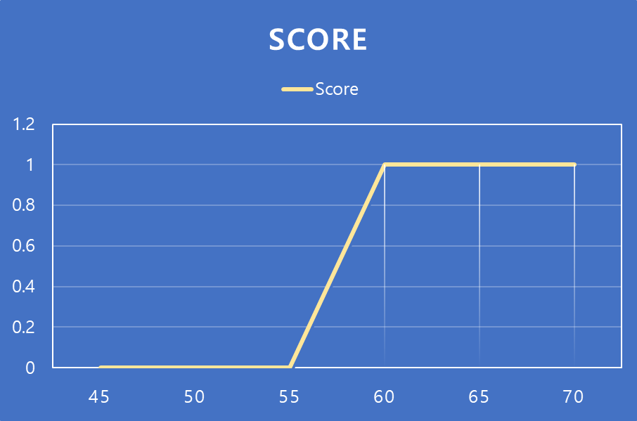
- 이러한 그래프는 Wx+b와 같은 함수가 아닌 S자 형태로 표현할 수 있는 함수가 필요하다.
- S자 모양의 함수 f를 설정하고 가설은 f(Wx+b)를 사용.(f : 시그모이드 함수)
1-1. Sigmoid Function
- Sigmoid function : 0~1 출력
- 가설은 아래와 같은 식으로 구성됨

- 선형 회귀에서는 W, b를 찾는 것이 목표 -> 여기서도 동일함 -> W, b는 시그모이드에 어떤 영향을 주나?
import numpy as np # 넘파이 사용
import matplotlib.pyplot as plt # 맷플롯립사용

def sigmoid(x): # 시그모이드 함수 정의
return 1/(1+np.exp(-x))- 1) W가 1이고 b가 0인 그래프
x = np.arange(-5.0, 5.0, 0.1)
y = sigmoid(x)

plt.plot(x, y, 'g')
plt.plot([0,0],[1.0,0.0], ':') # 가운데 점선 추가
plt.title('Sigmoid Function')
plt.show()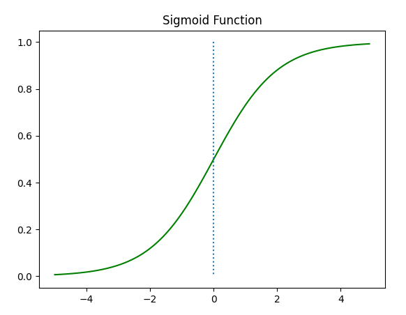
- 2) W 값 변화에 따른 그래프(빨간색 : W=0.5, 파란색 : W=2)
x = np.arange(-5.0, 5.0, 0.1)
y1 = sigmoid(0.5*x)
y2 = sigmoid(x)
y3 = sigmoid(2*x)

plt.plot(x, y1, 'r', linestyle='--') # W의 값이 0.5일때
plt.plot(x, y2, 'g') # W의 값이 1일때
plt.plot(x, y3, 'b', linestyle='--') # W의 값이 2일때
plt.plot([0,0],[1.0,0.0], ':') # 가운데 점선 추가
plt.title('Sigmoid Function')
plt.show()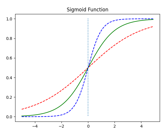
- W는 경사도를 결정(W가 클수록 경사도가 커짐 = W와 경사도는 비례함)
- 3) b값 변화에 따른 좌, 우 이동(빨간색 : x + 0.5, 초록색 : x + 1, 파란색 : x + 1.5)
x = np.arange(-5.0, 5.0, 0.1)
y1 = sigmoid(x+0.5)
y2 = sigmoid(x+1)
y3 = sigmoid(x+1.5)

plt.plot(x, y1, 'r', linestyle='--') # x + 0.5
plt.plot(x, y2, 'g') # x + 1
plt.plot(x, y3, 'b', linestyle='--') # x + 1.5
plt.plot([0,0],[1.0,0.0], ':') # 가운데 점선 추가
plt.title('Sigmoid Function')
plt.show()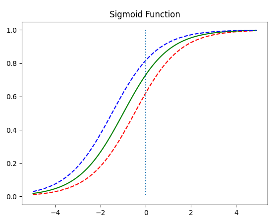
- 1 > b는 오른쪽, 1 < b는 왼쪽으로 이동시킴
- 시그모이드의 출력이 0~1 사이인것을 이용하여 0.5 이상은 True, 이하는 False로 판단
1-2. Cost function
- 선형 회귀에서 사용한 것처럼 MSE(평균 제곱 오차)를 사용(아래 식)

- 이 Cost Function을 미분하면 심한 비볼록 형태의 그래프가 됨
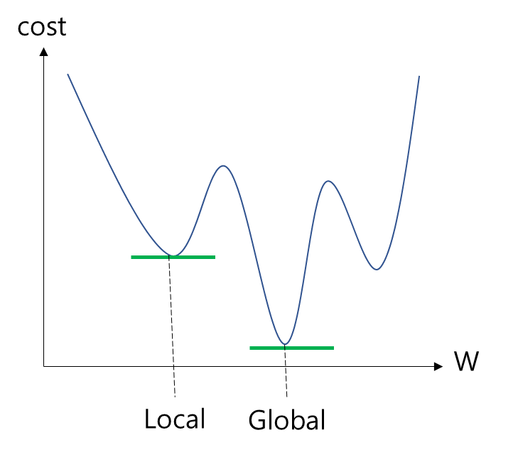
- 이때 경사하강법의 문제점 중 하나인 Local Minimum 문제가 발생할 수 있음.(목표는 Global Minimum인데 Local을 찾고 끝나는 것)
- 실제값이 1인데 예측값이 0인 경우와 실제값이 0인데 예측값이 1인 경우 오차가 커져야 함.
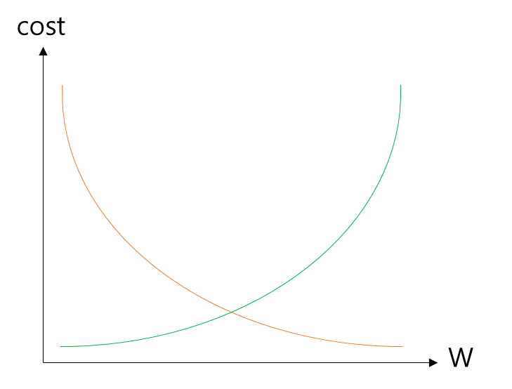
- 위 로그함수의 그래프가 그 조건을 만족
- 위 그래프는 각각 y가 1인지, 0인지에 따라 분리되어 있었지만 이를 하나로 합치면 아래와 같은 식이 된다.

- 이 식을 이제 MSE에 넣어서 오차 평균을 구한다.

- 위 cost function은 실제값 y와 예측값 H(x)의 차이가 커지면 cost가 커지고, 실제값 y와 예측값 H(x)의 차이가 작아지면 cost가 작아진다. -> 경사 하강법을 수행하면서 최적의 가중치 W를 찾아간다.

1-3. Logistic Regression with PyTorch
- 필요한 도구 임포트 및 랜덤 시드 고정
import torch
import torch.nn as nn
import torch.nn.functional as F
import torch.optim as optim

torch.manual_seed(1)- x_train과 y_train을 텐서로 선언
x_data = [[1, 2], [2, 3], [3, 1], [4, 3], [5, 3], [6, 2]]
y_data = [[0], [0], [0], [1], [1], [1]]
x_train = torch.FloatTensor(x_data)
y_train = torch.FloatTensor(y_data)- x_train과 y_train의 크기를 확인
print(x_train.shape)
print(y_train.shape)torch.Size([6, 2])
torch.Size([6, 1])- (6, 2), (6, 1)이므로 가중치 벡터의 크기는 (2, 1)이어야 함.
- x_train을 X, 가중치 벡터를 W라고 할 때, XW를 성립하기 위해서 가중치 벡터의 크기를 (2, 1)로 만들어야 함.
- 가설식은 아래와 같다.
hypothesis = 1 / (1 + torch.exp(-(x_train.matmul(W) + b)))- 위의 가설식은 파이토치에서 제공하는 시그모이드 함수를 통해 더 간단히 할 수 있음
hypothesis = torch.sigmoid(x_train.matmul(W) + b)- W와 b는 모두 0으로 초기화되어 시그모이드 후 출력값은 0.5임
print(hypothesis) # 예측값인 H(x) 출력tensor([[0.5000],
[0.5000],
[0.5000],
[0.5000],
[0.5000],
[0.5000]], grad_fn=<MulBackward>)- 비용 함수(예측값과 실제값 사이의 cost를 구하는 함수) 구현(한 원소에 대해서만)
-(y_train[0] * torch.log(hypothesis[0]) +
(1 - y_train[0]) * torch.log(1 - hypothesis[0]))tensor([0.6931], grad_fn=<NegBackward>)- 비용 함수(예측값과 실제값 사이의 cost를 구하는 함수) 구현(모든 원소에 대해서)
losses = -(y_train * torch.log(hypothesis) +
           (1 - y_train) * torch.log(1 - hypothesis))
print(losses)tensor([[0.6931],
[0.6931],
[0.6931],
[0.6931],
[0.6931],
[0.6931]], grad_fn=<NegBackward>)- 전체 오차에 대한 평균을 구함(MSE)
cost = losses.mean()
print(cost)tensor(0.6931, grad_fn=<MeanBackward1>)- PyTorch에서 제공하는 '교차 엔트로피'함수를 이용하는 것도 가능함
x_data = [[1, 2], [2, 3], [3, 1], [4, 3], [5, 3], [6, 2]]
y_data = [[0], [0], [0], [1], [1], [1]]
x_train = torch.FloatTensor(x_data)
y_train = torch.FloatTensor(y_data)
# 모델 초기화
W = torch.zeros((2, 1), requires_grad=True)
b = torch.zeros(1, requires_grad=True)
# optimizer 설정
optimizer = optim.SGD([W, b], lr=1)
nb_epochs = 1000
for epoch in range(nb_epochs + 1):
# Cost 계산
hypothesis = torch.sigmoid(x_train.matmul(W) + b)
cost = -(y_train * torch.log(hypothesis) +
(1 - y_train) * torch.log(1 - hypothesis)).mean()
# cost로 H(x) 개선
optimizer.zero_grad()
cost.backward()
optimizer.step()
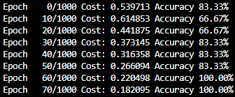
# 100번마다 로그 출력
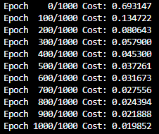
if epoch % 100 == 0:
print('Epoch {:4d}/{} Cost: {:.6f}'.format(
epoch, nb_epochs, cost.item()
))
- 예측값 확인
hypothesis = torch.sigmoid(x_train.matmul(W) + b)
print(hypothesis)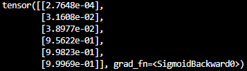
- 0.5를 넘기면 True, 넘지 않으면 False로 정해 출력
# 0.5보다 크면 True, 작으면 Fasle
prediction = hypothesis >= torch.FloatTensor([0.5])
print(prediction)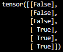
- 훈련 후 최적화 된 W, b값
# 최적화 된 W, b 값
print(W)
print(b)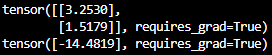
2. Logistic Regression with nn.Module
- 필요한 도구 임포트 및 랜덤 시드 설정
import torch
import torch.nn as nn
import torch.nn.functional as F
import torch.optim as optim

torch.manual_seed(1)- 훈련 데이터를 텐서로 선언
x_data = [[1, 2], [2, 3], [3, 1], [4, 3], [5, 3], [6, 2]]
y_data = [[0], [0], [0], [1], [1], [1]]
x_train = torch.FloatTensor(x_data)
y_train = torch.FloatTensor(y_data)- nn.Sequential() : nn.Module 층을 차례로 쌓게 해줌.
model = nn.Sequential(
   nn.Linear(2, 1), # input_dim = 2, output_dim = 1
   nn.Sigmoid() # 출력은 시그모이드 함수를 거친다
)print(model(x_train))- 그러나 W, b가 훈련 전 이므로 위 코드의 결과는 별 의미가 없음
# optimizer 설정
optimizer = optim.SGD(model.parameters(), lr=1)
nb_epochs = 1000
for epoch in range(nb_epochs + 1):
# H(x) 계산
hypothesis = model(x_train)
# cost 계산
cost = F.binary_cross_entropy(hypothesis, y_train)
# cost로 H(x) 개선
optimizer.zero_grad()
cost.backward()
optimizer.step()
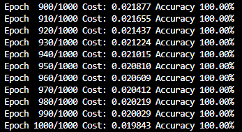
# 20번마다 로그 출력
if epoch % 10 == 0:
prediction = hypothesis >= torch.FloatTensor([0.5]) # 예측값이 0.5를 넘으면 True로 간주
correct_prediction = prediction.float() == y_train # 실제값과 일치하는 경우만 True로 간주
accuracy = correct_prediction.sum().item() / len(correct_prediction) # 정확도를 계산
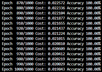
print('Epoch {:4d}/{} Cost: {:.6f} Accuracy {:2.2f}%'.format( # 각 에포크마다 정확도를 출력
epoch, nb_epochs, cost.item(), accuracy * 100,
))
print(list(model.parameters()))[Parameter containing:
tensor([[3.2534, 1.5181]], requires_grad=True), Parameter containing:
tensor([-14.4839], requires_grad=True)]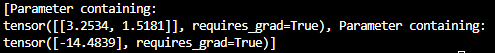
Logistic Regression with ANN
- 로지스틱 회귀는 인공 신경망으로 간주할 수 있다.
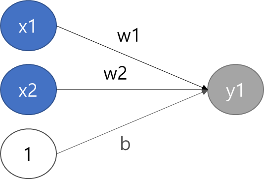
- 위 신경망은 다음과 같은 식으로 표현된다.

3. Logistic Regression with Class
import torch
import torch.nn as nn
import torch.nn.functional as F
import torch.optim as optim
torch.manual_seed(1)
x_data = [[1, 2], [2, 3], [3, 1], [4, 3], [5, 3], [6, 2]]
y_data = [[0], [0], [0], [1], [1], [1]]
x_train = torch.FloatTensor(x_data)
y_train = torch.FloatTensor(y_data)
class BinaryClassifier(nn.Module):
    def __init__(self):
        super().__init__()
        self.linear = nn.Linear(2, 1)
        self.sigmoid = nn.Sigmoid()

    def forward(self, x):
        return self.sigmoid(self.linear(x))
model = BinaryClassifier()
# optimizer 설정
optimizer = optim.SGD(model.parameters(), lr=1)

nb_epochs = 1000
for epoch in range(nb_epochs + 1):

    # H(x) 계산
    hypothesis = model(x_train)

    # cost 계산
    cost = F.binary_cross_entropy(hypothesis, y_train)

    # cost로 H(x) 개선
    optimizer.zero_grad()
    cost.backward()
    optimizer.step()

    # 20번마다 로그 출력
    if epoch % 10 == 0:
        prediction = hypothesis >= torch.FloatTensor([0.5]) # 예측값이 0.5를 넘으면 True로 간주
        correct_prediction = prediction.float() == y_train # 실제값과 일치하는 경우만 True로 간주
        accuracy = correct_prediction.sum().item() / len(correct_prediction) # 정확도를 계산
        print('Epoch {:4d}/{} Cost: {:.6f} Accuracy {:2.2f}%'.format( # 각 에포크마다 정확도를 출력
            epoch, nb_epochs, cost.item(), accuracy * 100,
        ))
출처 : 'PyTorch로 시작하는 딥 러닝 입문' <이 책의 내용을 요약 정리한 것임.>

매일 매일 새로워지는 나 자신을 꿈꾸며