LSTM을 활용한 주가 예측 모델링 (1)

프로젝트 내용

: yfinance (Yahoo finance)로부터 가져온 5년치 실시간 증권 데이터를 기반으로 미래 주가를 예측하는 프로젝트 진행 내용을 기록합니다.

github

git clone https://github.com/MachuEngine/tesla-lstm-predictor.git

---

1. Config

초기 Config 파일이다. 진행 과정에서 하이퍼 파라미터 튜닝 등을 통해 업데이트되어야 할 것 같다.

data:
  path: "./data"

train:
  num_epochs: 20
  learning_rate: 0.001
  input_size: 1
  hidden_size: 128
  num_layers: 3
  output_size: 1

model:
 pretrained: true

logging:
  level: INFO
  file: "./logs/train.log"

checkpoint:
  directory: "./checkpoints"
  save_interval: 5

2. main.py

모든 기능은 main함수에서 호출해서 처리되는 구조로 모듈화 되어있다.

import src.utils as utils
import src.dataset as dataset
import src.model as model
import src.train as train
import src.eval as eval
import src.visualization as visualization

def main(config):
    utils.setup_logging(config["logging"]["file"])
    
    train_loader, test_loader, scaler, data = dataset.dataset()
    
    lstm_model = model.LSTMModel(
        config["train"]["input_size"], 
        config["train"]["hidden_size"], 
        config["train"]["num_layers"], 
        config["train"]["output_size"])
    
    train.train_lstm_model(lstm_model, train_loader, config)

    predictions, actuals = eval.evaluate(lstm_model, test_loader, config)

    visualization.plot_predictions(predictions, actuals, scaler, data)

if __name__ == "__main__":
    config_path = "./configs/config.yaml"
    config = utils.load_config(config_path)
    main(config)

3. model.py

LSTM로 시퀀스 데이터가 입력되고 Fully connected layer의 출력을 통해 다음 데이터 예측 결과가 나오는 구조로 되어있다.

import torch
import torch.nn as nn

class LSTMModel(nn.Module):
    def __init__(self, input_size, hidden_size, num_layers, output_size, activation='relu'):
        super(LSTMModel, self).__init__()
        self.hidden_size = hidden_size
        self.num_layers = num_layers
        
        # LSTM 레이어 정의
        self.lstm = nn.LSTM(input_size, hidden_size, num_layers, batch_first=True)
        
        # 출력층 정의
        if activation == 'relu':
            self.fc = nn.Sequential(
                nn.Linear(hidden_size, output_size),
                nn.ReLU()  # 음수 값 방지
            )
        elif activation == 'sigmoid':
            self.fc = nn.Sequential(
                nn.Linear(hidden_size, output_size),
                nn.Sigmoid()  # 0 ~ 1 범위로 제한
            )
        else:  # 기본 활성화 함수 없음
            self.fc = nn.Linear(hidden_size, output_size)

    def forward(self, x):
        # 초기 은닉 상태 및 셀 상태 정의 (batch_size, hidden_size)
        h0 = torch.zeros(self.num_layers, x.size(0), self.hidden_size).to(x.device)
        c0 = torch.zeros(self.num_layers, x.size(0), self.hidden_size).to(x.device)
        
        # LSTM 순전파: out shape -> (batch, seq_length, hidden_size)
        out, _ = self.lstm(x, (h0, c0))
        
        # 마지막 타임스텝의 출력을 사용하여 예측
        out = self.fc(out[:, -1, :])
        return out

아래부터는 기능별로 모듈화된 함수이다.

4. dataset()

처음에는 일일 종가 데이터만 이용해서 미래 주가 예측을 하려고 한다. (data 정의 시 Close 컬럼만 다시 할당하여 사용) 이후에는 거래량을 포함해 좀 더 많은 feature를 사용해서 예측 결과를 비교 해보려고한다.

import numpy as np
import pandas as pd
import yfinance as yf
import matplotlib.pyplot as plt
import torch
import torch.nn as nn
from torch.utils.data import DataLoader, TensorDataset
from sklearn.preprocessing import MinMaxScaler

def dataset():
    # TSLA 주가 데이터 다운로드 (예: 최근 5년간의 일일 주가)
    ticker = "TSLA"
    data = yf.download(ticker, period="5y", interval="1d")
    data = data[['Close']]  # 종가만 사용

    # Train-test split (먼저 나눔)
    train_size = int(len(data) * 0.8)
    train_data = data[:train_size]
    test_data = data[train_size:]

    # 데이터 정규화 (훈련 데이터에 대해서만 fit, 테스트 데이터는 훈련 데이터 기반으로 fit한 정규화 기반으로 transform)
    scaler = MinMaxScaler(feature_range=(0, 1))
    scaled_train_data = scaler.fit_transform(train_data)  # 훈련 데이터에 대해 fit_transform
    scaled_test_data = scaler.transform(test_data)       # 테스트 데이터에 대해 transform

    # 시퀀스 데이터 준비 함수
    def create_sequences(dataset, time_step=120):
        X, y = [], []
        for i in range(len(dataset) - time_step - 1):
            X.append(dataset[i:(i + time_step), 0])
            y.append(dataset[i + time_step, 0])
        return np.array(X), np.array(y)

    time_step = 120
    X_train, y_train = create_sequences(scaled_train_data, time_step)
    X_test, y_test = create_sequences(scaled_test_data, time_step)

    # Tensor 변환 및 차원 추가
    X_train = torch.tensor(X_train, dtype=torch.float32).unsqueeze(-1)  # Add input_size dimension
    y_train = torch.tensor(y_train, dtype=torch.float32).unsqueeze(-1)  # Match output size with input
    X_test = torch.tensor(X_test, dtype=torch.float32).unsqueeze(-1)  # Add input_size dimension
    y_test = torch.tensor(y_test, dtype=torch.float32).unsqueeze(-1)  # Match output size with input

    print(f"y_train min: {y_train.min()}, max: {y_train.max()}")
    print(f"y_test min: {y_test.min()}, max: {y_test.max()}")

    # TensorDataset 및 DataLoader 생성
    train_dataset = TensorDataset(X_train, y_train)
    test_dataset = TensorDataset(X_test, y_test)

    batch_size = 32
    train_loader = DataLoader(train_dataset, batch_size=batch_size, shuffle=True, drop_last=True)
    test_loader = DataLoader(test_dataset, batch_size=batch_size, shuffle=False, drop_last=True)

    return train_loader, test_loader, scaler, data

5. train_lstm_model()

import numpy as np
import torch
import torch.nn as nn
from src.model import LSTMModel

def train_lstm_model(model, train_loader, config):
    # 모델 초기화
    model = LSTMModel(config["train"]["input_size"], config["train"]["hidden_size"], config["train"]["num_layers"], config["train"]["output_size"])

    # 장치 설정 (GPU 사용 가능 시 GPU 사용)
    device = torch.device("cuda" if torch.cuda.is_available() else "cpu")
    model.to(device)

    # MSE 대신 Huber Loss 사용
    criterion = nn.SmoothL1Loss()
    optimizer = torch.optim.Adam(model.parameters(), lr=config["train"]["learning_rate"])

    num_epochs = config["train"]["num_epochs"]

    for epoch in range(num_epochs):
        model.train()
        train_losses = []
        for batch_X, batch_y in train_loader:
            batch_X = batch_X.to(device)
            batch_y = batch_y.to(device)

            optimizer.zero_grad()
            outputs = model(batch_X)
            loss = criterion(outputs, batch_y)
            loss.backward()
            optimizer.step()

            train_losses.append(loss.item())

        # 에포크별 학습 손실 출력
        print(f"Epoch {epoch+1}/{num_epochs}, Loss: {np.mean(train_losses):.6f}")

6. evaluate()

import numpy as np
import torch

def evaluate(model, test_loader, config):
    device = torch.device("cuda" if torch.cuda.is_available() else "cpu")
    model.to(device)
    model.eval()

    predictions = []
    actuals = []
    with torch.no_grad():
        for batch_X, batch_y in test_loader:
            # Ensure batch_X and batch_y are tensors
            batch_X, batch_y = batch_X.to(device), batch_y.to(device)

            # Forward pass
            outputs = model(batch_X)
            predictions.append(outputs.cpu().numpy())
            actuals.append(batch_y.cpu().numpy())

    return np.concatenate(predictions), np.concatenate(actuals)

7. plot_predictions()

import matplotlib.pyplot as plt

def plot_predictions(predictions, actuals, scaler, data):
    """
    예측값과 실제값을 시각화하는 함수.

    Args:
        predictions (ndarray): 예측된 값 (Test 데이터셋 기반).
        actuals (ndarray): 실제 값 (Test 데이터셋 기반).
        scaler (MinMaxScaler): 데이터 스케일링에 사용된 스케일러.
        data (DataFrame): 원본 데이터셋.
    """
    print(f"Predictions before inverse transform: {predictions[:10]}")


    # 예측값과 실제값 스케일 복원
    predictions = scaler.inverse_transform(predictions.reshape(-1, 1))
    actuals = scaler.inverse_transform(actuals.reshape(-1, 1))

    # 테스트 데이터가 시작하는 인덱스
    test_start_idx = len(data) - len(predictions)

    print(f"Original data range: {data['Close'].min()} to {data['Close'].max()}")
    print(f"Predictions range after inverse transform: {predictions.min()} to {predictions.max()}")
    print(f"Actuals range after inverse transform: {actuals.min()} to {actuals.max()}")


    # 시각화
    plt.figure(figsize=(12, 6))
    plt.plot(data.index, data["Close"], label="Original Data", alpha=0.7)
    plt.plot(data.index[test_start_idx:], predictions, label="Predictions", color="red", linestyle="--")
    plt.plot(data.index[test_start_idx:], actuals, label="Actuals", color="green", linestyle="--")
    plt.title("Price Prediction")
    plt.xlabel("Time")
    plt.ylabel("Price")
    plt.legend()
    plt.show()

8. load_config() , setup_logging()

import yaml
import logging
import os

def load_config(config_path):
    with open(config_path, 'r', encoding="utf-8") as f:
        config = yaml.safe_load(f)
    return config

def setup_logging(log_file, level=logging.INFO):
    os.makedirs(os.path.dirname(log_file), exist_ok=True)
    logging.basicConfig(
        level=level,
        format="%(asctime)s [%(levelname)s] %(message)s",
        handlers=[
            logging.FileHandler(log_file),
            logging.StreamHandler()
        ]
    )

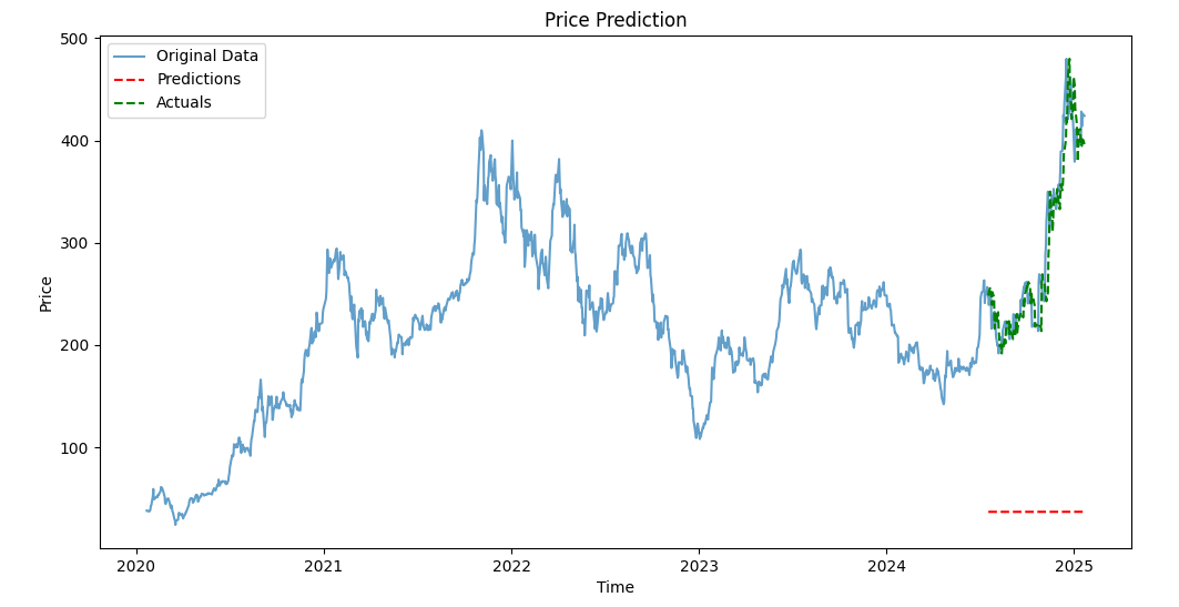
9. RESULT

아래 결과를 보면 Predictions의 정규화 해제 후 범위가 매우 좁게 출력되어 예측값이 actuals와 매우 다르게 보인다. 해당 문제가 정규화 문제인지, 학습 부족으로 인한 문제인지 해결 되어야할 것 같다.

(stt_env) C:\Users\Admin\Documents\Projects\tesla-lstm-predictor>python main.py
[*********************100%***********************]  1 of 1 completed

[정규화 후 Data의 MinMax]
y_train min: 0.17503666877746582, max: 1.0
y_test min: 0.4345259964466095, max: 1.1811143159866333

[Training]
Epoch 1/20, Loss: 0.028938
Epoch 2/20, Loss: 0.009924
Epoch 3/20, Loss: 0.004380
Epoch 4/20, Loss: 0.002077
Epoch 5/20, Loss: 0.001540
Epoch 6/20, Loss: 0.001432
Epoch 7/20, Loss: 0.001276
Epoch 8/20, Loss: 0.001177
Epoch 9/20, Loss: 0.000965
Epoch 10/20, Loss: 0.000959
Epoch 11/20, Loss: 0.000840
Epoch 12/20, Loss: 0.000751
Epoch 13/20, Loss: 0.000764
Epoch 14/20, Loss: 0.000731
Epoch 15/20, Loss: 0.000661
Epoch 16/20, Loss: 0.000632
Epoch 17/20, Loss: 0.000606
Epoch 18/20, Loss: 0.000569
Epoch 19/20, Loss: 0.000631
Epoch 20/20, Loss: 0.000650

[정규화를 해제한 후 예측 결과]
Predictions before inverse transform: [[0.03307568]
 [0.03306588]
 [0.03306002]
 [0.03305848]
 [0.03305592]
 [0.03305326]
 [0.03304786]
 [0.03304686]
 [0.03304674]
 [0.03303646]]
 
[정규화를 해제한 후 data, predictions, actuals의 MinMax]
Original data range: Ticker
TSLA    24.081333
dtype: float64 to Ticker
TSLA    479.859985
dtype: float64
Predictions range after inverse transform: 36.8167610168457 to 36.90672302246094
Actuals range after inverse transform: 191.75999450683594 to 479.8599548339844

빨간색 점선이 predictions 라인인데, 주가를 전혀 반영해주지 못하고 있음을 plot으로도 확인할 수 있다.