자동차 번호판 인식 with OpenCV
1. 라이브러리 호출
import cv2
import numpy as np
import matplotlib.pyplot as plt
import pytesseract
plt.style.use('dark_background')
사용한 라이브러리들은 총 4가지이다.
사용 용도는 다음과 같다.
cv2 : Opencv
numpy : 복잡한 수치계산
matplotlib : 시각화
pytesseract : 글자 인식 (사진에서 번호판 숫자 추출)
2. Read Input Image
2번째 단계에서는 이미지를 불러온 후 너비, 높이, 채널의 값을 저장한다.
matplotlib을 이용해 정상적으로 불러왔는지 출력해보고 저장된 너비, 높이, 채널을 확인한다.
img_ori = cv2.imread('car2.png')

height, width, channel = img_ori.shape

plt.figure(figsize=(12, 10))
plt.imshow(img_ori,cmap='gray')
print(height, width, channel)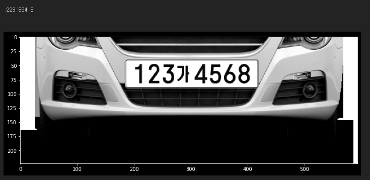
높이가 223, 너비가 594, 채널이 3 (RGB 이므로 3)인 것을 알 수 있다.
출력을 할 때 cmap을 gray로 설정했음에도 육안으로는 원본 사진과 큰 차이를 볼 순 없었다.
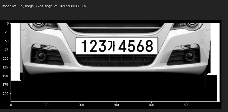
3. Convert Image to Grayscale
위에서는 gray로 출력만 해보았을 뿐 실제로 변환한 것은 아니다.
3번째 단계에서는 opencv의 cvtColor 메소드를 이용해 RGB를 GRAY로 변환한다.
변환하는 방법은 2가지이다.
gray = cv2.cvtColor(img_ori, cv2.COLOR_BGR2GRAY)
plt.figure(figsize=(12,10))
plt.imshow(gray, cmap='gray')
hsv = cv2.cvtColor(img_ori, cv2.COLOR_BGR2HSV)
gray = hsv[:, :, 2]
plt.figure(figsize=(12,10))
plt.imshow(gray, cmap='gray')
위 두 코드의 동작은 완전히 동일하므로 마음에 드는 것으로 작성하면 된다.
출력 결과는 아래와 같다.
4. Adaptive Thresholding
Thresholding을 해주기 전에 가우시안 블러를 해주는 것이 번호판을 더 잘 찾게 만들어 줄 수 있다.
가우시안 블러는 사진의 노이즈를 없애는 작업이다.
가우시안 블러를 적용해야하는 이유는 아래 4-1에서 설명한다.
그럼 먼저 Thresholding을 살펴보자.
Thresholding 이란 지정한 threshold 값을 기준으로 정하고
이보다 낮은 값은 0, 높은 값은 255로 변환한다. 즉 흑과 백으로만 사진을 구성하는 것이다.
이걸 해주는 이유는 5번째 단계에서 Contours를 찾으려면 검은색 배경에 흰색 바탕이어야 한다.
또 육안으로 보기에도 객체를 더 뚜렷하게 볼 수 있다.
아래 Thresholding을 적용한 사진을 보면 이해가 쉽다.
img_blurred = cv2.GaussianBlur(gray, ksize=(5, 5), sigmaX=0)
img_blur_thresh = cv2.adaptiveThreshold(
img_blurred,
maxValue=255.0,
adaptiveMethod=cv2.ADAPTIVE_THRESH_GAUSSIAN_C,
thresholdType=cv2.THRESH_BINARY_INV,
blockSize=19,
C=9
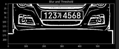
)4-1. Gaussian Blur 비적용 / 적용 비교
Thresholding 적용을 보았으니 가우시안 블러를 사용하는 이유를 알기위해
적용했을 때와 적용하지 않았을 때를 출력해본다.
img_thresh = cv2.adaptiveThreshold(
    gray,
    maxValue=255.0,
    adaptiveMethod=cv2.ADAPTIVE_THRESH_GAUSSIAN_C,
    thresholdType=cv2.THRESH_BINARY_INV,
    blockSize=19,
    C=9
)
plt.figure(figsize=(20,20))
plt.subplot(1,2,1)
plt.title('Threshold only')
plt.imshow(img_thresh, cmap='gray')
plt.subplot(1,2,2)
plt.title('Blur and Threshold')
plt.imshow(img_blur_thresh, cmap='gray')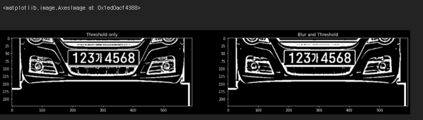
왼쪽이 가우시안 블러를 적용하지 않은 사진, 오른쪽이 적용한 사진이다.
언뜻보기엔 큰 차이를 못느낄 수 있지만 번호판 밑부분을 보면 좀 더 검은색 부분이 많아졌다.
5. Find Contours
Contours란 동일한 색 또는 동일한 강도를 가지고 있는 영역의 경계선을 연결한 선이다.
findContours()는 이런 Conturs들을 찾는 opencv 메소드이다.
위 메소드는 검은색 바탕에서 흰색 대상을 찾는다.
그래서 4번째 단계에서 Thresholding을 해주고 가우시안 블러를 적용해준 것이다.
그런데 공식문서에는 findCountours의 리턴 값으로
image, contours, hierachy 이렇게 3개가 나온다고 나와있지만
현재 첫번째 리턴 값인 image가 사라진 듯하다.
그래서 contours와 로 리턴을 받았다. hierachy는 쓸 일이 없어 로 받음
사진의 윤곽선을 모두 딴 후 opencv의 drawContours() 메소드로
원본사진이랑 크기가 같은 temp_result란 변수에 그려보았다
contours, _ = cv2.findContours(
    img_blur_thresh,
    mode=cv2.RETR_LIST,
    method=cv2.CHAIN_APPROX_SIMPLE
)

temp_result = np.zeros((height, width, channel), dtype=np.uint8)

cv2.drawContours(temp_result, contours=contours, contourIdx=-1, color=(255,255,255))

plt.figure(figsize=(12, 10))
plt.imshow(temp_result)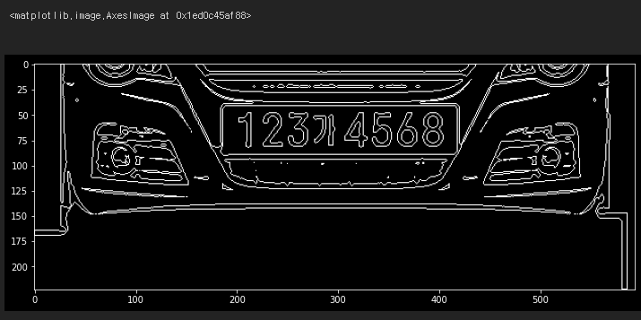
Contours를 찾아서 그린 결과를 볼 수 있다.
6. Prepare Data
원본 사진과 동일한 크기에다가 찾은 Countours들의 좌표를 이용해
사각형 형태로 그려본다. 동시에 딕셔너리를 하나 만들어 contours들의 정보를 저장한다.
temp_result = np.zeros((height, width, channel), dtype=np.uint8)

contours_dict = []

for contour in contours:
    x, y, w, h = cv2.boundingRect(contour)
    cv2.rectangle(temp_result, pt1=(x,y), pt2=(x+w, y+h), color=(255,255,255), thickness=2)

    contours_dict.append({
        'contour': contour,
        'x': x,
        'y': y,
        'w': w,
        'h': h,
        'cx': x + (w / 2),
        'cy': y + (h / 2)
    })

plt.figure(figsize=(12,10))
plt.imshow(temp_result, cmap='gray')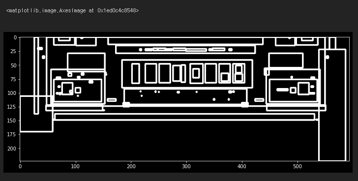
찾은 모든 Contours들을 사격형 형태로 볼 수 있다.
7. Select Candidates by Char Size
이제 번호판 글자인 것 같은 Contours들을 추려내야한다.
많은 방법이 있겠지만 단순히 생각해서
번호판의 숫자들을 손글씨처럼 다 다르지 않고 일정한 비율을 가진다.
때문에 이 비율을 이용하면 대충은 번호판 같은 contours들을 추려낼 수 있다.
아래 코드에서는 최소 비율을 0.25와 최대 비율을 1.0으로 설정한 후
contours의 너비와 높이를 이용해 비율을 구하고
우리가 정한 기준에 맞는 contours들만 따로 저장하였다.
MIN_AREA = 80
MIN_WIDTH, MIN_HEIGHT=2, 8
MIN_RATIO, MAX_RATIO = 0.25, 1.0

possible_contours = []

cnt = 0
for d in contours_dict:
    area = d['w'] * d['h']
    ratio = d['w'] / d['h']

    if area > MIN_AREA \
    and d['w'] > MIN_WIDTH and d['h'] > MIN_HEIGHT \
    and MIN_RATIO < ratio < MAX_RATIO:
        d['idx'] = cnt
        cnt += 1
        possible_contours.append(d)

temp_result = np.zeros((height, width, channel), dtype = np.uint8)

for d in possible_contours:
    cv2.rectangle(temp_result, pt1=(d['x'], d['y']), pt2=(d['x']+d['w'], d['y']+d['h']), color=(255, 255, 255), thickness=2)

plt.figure(figsize=(12, 10))
plt.imshow(temp_result, cmap='gray')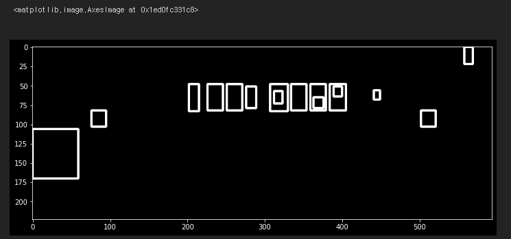
위 사진은 추려낸 contours들이다.
번호판 위치에 contours들이 선별된 걸 볼 수 있지만
전혀 관련 없는 영역의 contours들도 저장되었다.
이제 더 기준을 강화하여 번호판 글자들을 찾아야한다.
8. Select Candidates by Arrangement of Contours
8번째 단계에서는 남은 contours 중에 확실하게 번호판을 찾기 위해 기준을 강화한다.
번호판의 특성을 고려했을 때 세울 수 있는 기준은 아래와 같다.
- 번호판 Contours의 width와 height의 비율은 모두 동일하거나 비슷하다.
- 번호판 Contours 사이의 간격은 일정하다.
- 최소 3개 이상 Contours가 인접해 있어야한다. (대한민국 기준)
이 특성들을 고려하여 아래와 같이 코드를 작성한다.
최종적으로 얻어야 할 것은 번호판에 대한 후보군이다.
MAX_DIAG_MULTIPLYER = 5
MAX_ANGLE_DIFF = 12.0
MAX_AREA_DIFF = 0.5
MAX_WIDTH_DIFF = 0.8
MAX_HEIGHT_DIFF = 0.2
MIN_N_MATCHED = 3

def find_chars(contour_list):
    matched_result_idx = []

    for d1 in contour_list:
        matched_contours_idx = []
        for d2 in contour_list:
            if d1['idx'] == d2['idx']:
                continue

            dx = abs(d1['cx'] - d2['cx'])
            dy = abs(d1['cy'] - d2['cy'])

            diagonal_length1 = np.sqrt(d1['w'] ** 2 + d1['h'] ** 2)

            distance = np.linalg.norm(np.array([d1['cx'], d1['cy']]) - np.array([d2['cx'], d2['cy']]))
            if dx == 0:
                angle_diff = 90
            else:
                angle_diff = np.degrees(np.arctan(dy / dx))
            area_diff = abs(d1['w'] * d1['h'] - d2['w'] * d2['h']) / (d1['w'] * d1['h'])
            width_diff = abs(d1['w'] - d2['w']) / d1['w']
            height_diff = abs(d1['h'] - d2['h']) / d1['h']

            if distance < diagonal_length1 * MAX_DIAG_MULTIPLYER \
            and angle_diff < MAX_ANGLE_DIFF and area_diff < MAX_AREA_DIFF \
            and width_diff < MAX_WIDTH_DIFF and height_diff < MAX_HEIGHT_DIFF:
                matched_contours_idx.append(d2['idx'])

        matched_contours_idx.append(d1['idx'])

        if len(matched_contours_idx) < MIN_N_MATCHED:
            continue

        matched_result_idx.append(matched_contours_idx)

        unmatched_contour_idx = []
        for d4 in contour_list:
            if d4['idx'] not in matched_contours_idx:
                unmatched_contour_idx.append(d4['idx'])

        unmatched_contour = np.take(possible_contours, unmatched_contour_idx)

        recursive_contour_list = find_chars(unmatched_contour)

        for idx in recursive_contour_list:
            matched_result_idx.append(idx)

        break

    return matched_result_idx

result_idx = find_chars(possible_contours)

matched_result = []
for idx_list in result_idx:
    matched_result.append(np.take(possible_contours, idx_list))

temp_result = np.zeros((height, width, channel), dtype=np.uint8)

for r in matched_result:
    for d in r:
        cv2.rectangle(temp_result, pt1=(d['x'], d['y']), pt2=(d['x']+d['w'], d['y']+d['h']), color=(255,255,255), thickness=2)

plt.figure(figsize=(12, 10))
plt.imshow(temp_result, cmap='gray')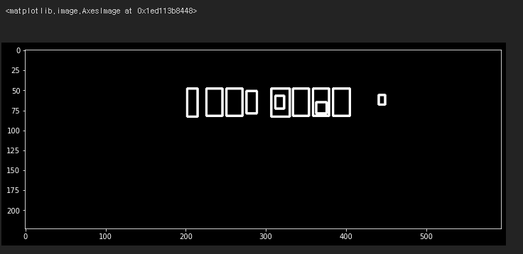
출력 결과는 번호판으로 추정되는 후보군이며
원본과 비교했을 때 번호판 부분임을 확인할 수 있다.
9. Rotate Plate Images
현재 우리 사진은 자동차가 정방향에서 찍혔기 때문에 번호판이 가지런하지만
대부분의 사진에서는 번호판이 기울어진 경우가 많을 것이다.
때문에 pytesseract를 이용하여 번호판 글자를 인식하기 위해
번호판 부분을 정방향으로 만들어 줄 필요가 있다.
9번째 단계에서는 해당 작업을 수행한다.
먼저 단계에서 얻은 모든 후보군에 대해 Affine Transform을 적용한다.
이후 번호판 부분만 Crop 하여 출력한다.
코드가 길기 때문에 Github 코드 참고!
보면 2개의 후보군이 출력된 걸 볼 수 있고 모두 정방향으로 잘 보인다.
10. Another Thresholding
하지만 만약 9번째 단계에서 번호판 Contours 가 없었을 때를 대비하여
10번째 단계에서는 처음에 선별되지 못한 Contours에 대해서도 후보군을 추린다.
로직은 위에서 했던 것과 동일하다.
longest_idx, longest_text = -1, 0
plate_chars = []

for i, plate_img in enumerate(plate_imgs):
    plate_img = cv2.resize(plate_img, dsize=(0, 0), fx=1.6, fy=1.6)
    _, plate_img = cv2.threshold(plate_img, thresh=0.0, maxval=255.0, type=cv2.THRESH_BINARY | cv2.THRESH_OTSU)

    # find contours again (same as above)
    contours, _ = cv2.findContours(plate_img, mode=cv2.RETR_LIST, method=cv2.CHAIN_APPROX_SIMPLE)

    plate_min_x, plate_min_y = plate_img.shape[1], plate_img.shape[0]
    plate_max_x, plate_max_y = 0, 0

    for contour in contours:
        x, y, w, h = cv2.boundingRect(contour)

        area = w * h
        ratio = w / h

        if area > MIN_AREA \
        and w > MIN_WIDTH and h > MIN_HEIGHT \
        and MIN_RATIO < ratio < MAX_RATIO:
            if x < plate_min_x:
                plate_min_x = x
            if y < plate_min_y:
                plate_min_y = y
            if x + w > plate_max_x:
                plate_max_x = x + w
            if y + h > plate_max_y:
                plate_max_y = y + h

    img_result = plate_img[plate_min_y:plate_max_y, plate_min_x:plate_max_x]
11. Find Chars
이제 11번째 단계에서는 추린 후보군을 이용하여 글자를 찾는다.
pytesseract를 사용해야 하는데 몇 가지 사전 준비가 필요하다.
- 먼저 tesseract를 다운받는다.
공식 다운로드 사이트 : 공식 사이트에서 다운받으면 2시간 가량 소요된다;;
시간을 단축하고 싶다면 어떤 분이 분할 압축하여 올려 놓은 아래 깃에 가서 다운받자.
tesseract 분할 압축 Gittesseract를 다운받은 경로를 기억해야한다.
나는 하드디스크(D 드라이브)에 다운받았다.
오른쪽 사이트에서 trained data 데이터를 다운받는다 -> trained data
다운받은 tesseart 경로에 tessdata에 trained data를 옮겨준다.
아래 코드를 pytesseract.image_to_string() 메소드 위에 추가한다.
pytesseract.pytesseract.tesseract_cmd = '본인 tesseract 경로/tesseract.exe'
이렇게 하면 pytesseract를 사용할 준비를 마쳤다.
이제 아래와 같이 코드를 작성 후 실행하고 결과를 출력한다.
    img_result = cv2.GaussianBlur(img_result, ksize=(3, 3), sigmaX=0)
    _, img_result = cv2.threshold(img_result, thresh=0.0, maxval=255.0, type=cv2.THRESH_BINARY | cv2.THRESH_OTSU)
    img_result = cv2.copyMakeBorder(img_result, top=10, bottom=10, left=10, right=10, borderType=cv2.BORDER_CONSTANT, value=(0,0,0))

    pytesseract.pytesseract.tesseract_cmd = 'D:/tesseract/tesseract.exe'
    chars = pytesseract.image_to_string(img_result, lang='kor', config='--psm 7 --oem 0')

    result_chars = ''
    has_digit = False
    for c in chars:
        if ord('가') <= ord(c) <= ord('힣') or c.isdigit():
            if c.isdigit():
                has_digit = True
            result_chars += c

    print(result_chars)
    plate_chars.append(result_chars)

    if has_digit and len(result_chars) > longest_text:
        longest_idx = i

    plt.subplot(len(plate_imgs), 1, i+1)
    plt.imshow(img_result, cmap='gray')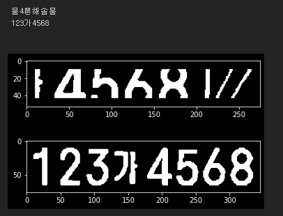
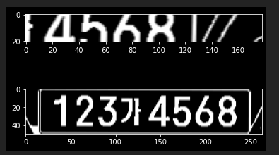
2개의 후보군을 문자로 변환하였을 때 위에건 이상한 글자가 출력되었고
아래건 정확하게 출력된 걸 확인할 수 있다.
코드에서 특수문자 나오거나 이상한 문자가 나올 경우 걸러주는 코드를 작성해줬기 때문에
최종적으로는 아래의 후보가 최종 번호판으로 선정된다.
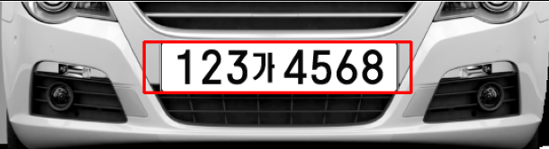
12. Result
이제 우리는 최종 번호판 좌표를 얻었으니 원본 이미지에 cv2.rectangle() 메소드를 이용해
사각형을 그린 후 출력을 하면 끝난다.
아래와 같이 코드 작성 후 출력해보자.
info = plate_infos[longest_idx]
chars = plate_chars[longest_idx]

print(chars)

img_out = img_ori.copy()

cv2.rectangle(img_out, pt1=(info['x'], info['y']), pt2=(info['x']+info['w'], info['y']+info['h']), color=(255,0,0), thickness=2)

cv2.imwrite(chars + '.jpg', img_out)

plt.figure(figsize=(12, 10))
plt.imshow(img_out)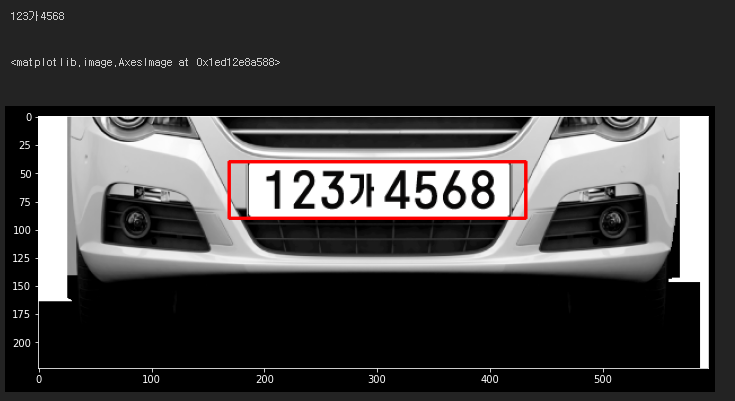
번호판이 아주 잘 인식되어 텍스트로 변환되었고
주변에 rectangle도 잘 나온 것을 확인할 수 있다.

링크해갑니다~