딥러닝 (2)

Chapter 2 텐서플로우 기초

텐서플로우와 케라스란

• 탠서플로우 (Tensorflow)
  -> 구글에서 유지/보수하는 오픈소스 딥러닝 프레임워크
  -> 파이썬을 기본으로 자바스크립트, 모바일, 에지 디바이스, REST API 등 다양한 개발 및 배포 환경 제공
  -> 퍼포먼스와 사용성 겸비한 프레임워크
  -> C++과 CUDA 기반으로 구현되어 뛰어난 퍼포먼스
  -> 2.x 버전의 즉시 실행(eager execution) 기능으로 사용성 향상

• 케라스 (Keras)
  -> 텐서플로우, 티아노(theano), CNTK를 백엔드로 하는 고차원(high-level) 딥러닝 프레임워크
  -> 텐서플로우 API에 흡수되면서 tf.slim과 tf.layers를 대체하는 핵심 구성요소로 자리잡음
  -> tf.slim, tf.layers – 텐서플로우 1버전에서 사용성을 높이기 위해제안되었던 고차원 모듈
  -> 텐서플로우와 함께 사용할 경우 매우 높은 편리성과 자유도 제공
  -> 루틴에 해당하는 부분은 케라스로 간편하고 신속하게 구현
  -> 커스텀 계층 등 저차원 구현은 텐서플로우를 이용하여 구현
  

텐서(Tensor)

• 텐서플로우의 기본 자료형
  -> NumPy의 array와 유사하나, 텐서플로우 내부에서 동작
  -> NumPy array와 텐서는 상호 변경 가능
  -> 텐서에는 다양한 연산(operation)을 적용할 수 있으며, 텐서플로우에서 연산의 최적화를 지원

텐서 슬라이싱

• Python의 리스트, NumPy의 array와 유사하게 슬라이싱 가능
  -> NumPy array처럼 기본적으로 pass-by-reference로 동작

변수 (Variables)

• 텐서플로우의 변수는 수학에서의 변수처럼 동작한다.
• 변수의 다양한 용도
  -> 학습 결과인 매개변수를 저장하기 위해 사용(trainable variable)
  -> 상태나 상수 등을 저장하기 위해 사용(non-trainable variable)
  -> 디버깅이나 연구를 위해 중간 계산 과정을 저장하는 임시 변수

그래프와 오토그래프

• 그래프 (tf.Graph)
  -> 텐서플로우 연산(tf.Operation)과 텐서(tf.Tensor)의 집합으로 이루어진 객체
  -> 텐서플로우 코어가 동작하는 단위로, 그래프에 대해서 연산 최적화가 이루어짐

• 오토그래프 (AutoGraph)
  -> @tf.function 데코레이터를 이용하면 파이썬 함수를 텐서플로우 그래프로 간편하게 변환할 수 있음

• 텐서보드 (Tensorboard)
  -> 텐서플로우의 동작을 요약해서 보여주는 도구
  -> 텐서플로우의 그래프를 시각화하여 보여주는 기능이 있음

모델의 정의

• 객체지향 형식의 모델 표현 방법
  -> 모델에 포함되는 변수, 계층 등을 '__ init__'함수에서 정의
  -> '__call__' 함수에서 네트워크의 정방향(feed-forward) 연산 정의
  -> 사전에 정의된 계층을 이용하는 것이 권장됨

모델의 학습

• 네트워크를 학습하기 위해 필요한 추가 정보
  -> 손실 함수(loss function)
  -> 최적화 방법(optimizer)
  -> 학습 데이터(training data)

import tensorflow as tf
import matplotlib.pyplot as plt

class LinearRegression(tf.Module):
    def __init__(self, **kwargs):   # defines variables and layers
        super().__init__(**kwargs)  # calls constructor of tf.Module
        self.w = tf.Variable(1.0, trainable=True, dtype=tf.float32, name='weight')  # weight variable
        self.b = tf.Variable(0.0, trainable=True, dtype=tf.float32, name='bias')    # bias variable

    def __call__(self, x):          # defines feed-forward operation
        return self.w * x + self.b  # y = w*x + b (linear regression)
        
model = LinearRegression()

def loss_func(y_true, y_pred):                           # defines loss function
    return tf.losses.mean_squared_error(y_true, y_pred)  # loss function for least squares
    
x = tf.random.normal([1000])      # x drawn from Gaussian distribution
noise = tf.random.normal([1000])  # noise drawn from Gaussian distribution
w = 10.0                          # groundtruth weight
b = 3.0                           # groundtruth bias
y = w * x + b + noise             # dataset

plt.scatter(x, y)
plt.show()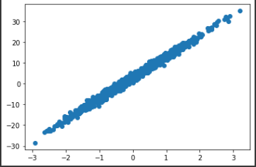

y_pred = model(x)  # get output from initialized model

plt.scatter(x, y)
plt.plot(x, y_pred, 'r-')
plt.show()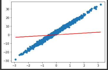

def train_step(model, x, y, learning_rate):  # training step
    with tf.GradientTape() as t:     # calculates gradient in this context
        y_pred = model(x)            # feed-forward calculation
        loss = loss_func(y, y_pred)  # loss calculation w/ groundtruth
    dw, db = t.gradient(loss, [model.w, model.b])  # get gradients of weight and bias

    model.w.assign_sub(learning_rate * dw)  # apply gradient-descent on weight  w = w - (learning_rate * dw)
    model.b.assign_sub(learning_rate * db)  # apply gradient-descent on bias    b = b - (learning_rate * db)
    return loss                             # returns loss for observing progress
    
w_hist = [model.w.numpy()]  # collect history of weight
b_hist = [model.b.numpy()]  # collect history of bias
for epoch in range(20):  # total 20 epochs(iterations)
    loss = train_step(model, x, y, 0.1)  # train one step
    w_hist.append(model.w.numpy())       # collect updated weight
    b_hist.append(model.b.numpy())       # collect updated bias
    print('epoch {}, loss={}'.format(epoch+1, loss))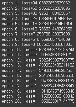    

plt.plot(w_hist, 'r-', label='w')  # history of weight
plt.plot(b_hist, 'b-', label='b')  # history of bias
plt.legend()

plt.plot([10.0 for _ in range(len(w_hist))], 'r--')  # groundtruth of weight 
plt.plot([3.0 for _ in range(len(b_hist))], 'b--')   # groundtruth of bias
plt.show()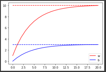

plt.plot(w_hist, b_hist, 'ko-')  # scatter plot in feature space
plt.plot([10.0], [3.0], 'ro')    # groundtruth marked in red
plt.xlabel('weight')
plt.ylabel('bias')
plt.show()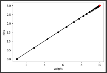

plt.scatter(x, y)            # scatter plot training samples
plt.plot(x, model(x), 'r-')  # plot prediction by red line
plt.show()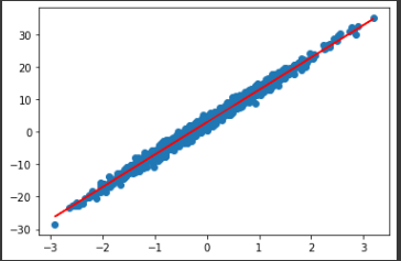

케라스를 이용한 모델의 학습

• 케라스 API를 이용

import tensorflow as tf
import matplotlib.pyplot as plt

class LinearRegression(tf.keras.Model):
    def __init__(self, **kwargs):
        super().__init__(**kwargs)
        self.w = tf.Variable(1.0)
        self.b = tf.Variable(0.0)
    
    def call(self, x):
        return self.w * x + self.b
        
model = LinearRegression()

x = tf.random.normal([1000])
noise = tf.random.normal([1000])
w = 10.0
b = 3.0
y = w * x + b + noise

model.compile(optimizer=tf.keras.optimizers.SGD(0.1),
              loss=tf.keras.losses.MeanSquaredError())

model.fit(x, y, epochs=20, batch_size=1000)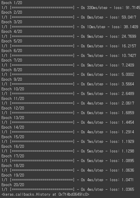

plt.scatter(x, y)
plt.show()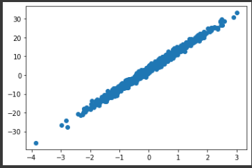

plt.scatter(x, y)
plt.plot(x, model(x), 'r-')
plt.show()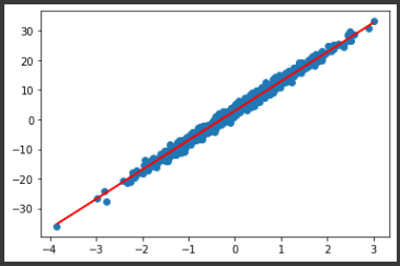

이 글은 제로베이스 데이터 취업 스쿨의 강의 자료 일부를 발췌하여 작성되었습니다