[알고리즘] Divide-and-Conquer (분할 정복)

hye0n.gyu·2023년 2월 1일

알고리즘

목록 보기

2/6

⭐Divide-and-Conquer(분할 정복)란?

여러 알고리즘의 기본이 되는 해결방법으로, 기본적으로는 엄청나게 크고 방대한 문제를 조금씩 조금씩 나눠가면서 용이하게 풀 수 있는 문제 단위로 나눈 다음 그것들을 다시 합쳐서 해결하자는 개념
분할 (Divide)
- 해결하기 쉽도록 문제를 여러 개의 작은 부분으로 나눈다.
정복 (Conquer – Solve)
- 나눈 작은 문제를 각각 해결한다.
통합 (Combine – Obtain the solution)
- (필요하다면) 해결된 해답을 모은다.

Top down(하향식) approach

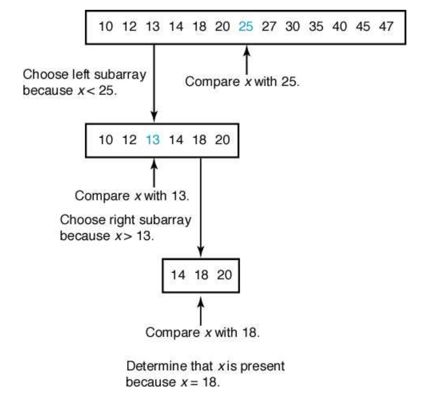
설계 전략

x가 배열의 중간에 위치하고 있는 항목과 같으면, “빙고”, 찾았다!
그렇지 않으면:

Divide (분할): 배열을 반으로 나누어서
x가 중앙에 위치한 항목보다 작으면 왼쪽 배열 반쪽을 선택,
그렇지 않으면 오른쪽 배열 반쪽을 선택한다.
Conquer (정복): 선택된 반쪽 배열에서 x를 찾는다.
Obtain the solution (or Combine 통합): (필요 없음)

 index location (index low, index high) { index mid;
   if (low > high)
      return 0;
else {
mid = (low + high) / 2; 
// 찾지 못했음
// 정수 나눗셈 (나머지 버림 - 내림)
// 찾았음
// 왼쪽 반을 선택함 // 오른쪽 반을 선택함
else
} }
return location(mid+1, high);
if (x == S[mid])
    return mid;
else if (x < S[mid])
return location(low, mid-1);
...
locationout = location(1, n);       // evoke location
...

시간 복잡도 W(n) = $lg$ n

⭐Merge Sort(합병 정렬)

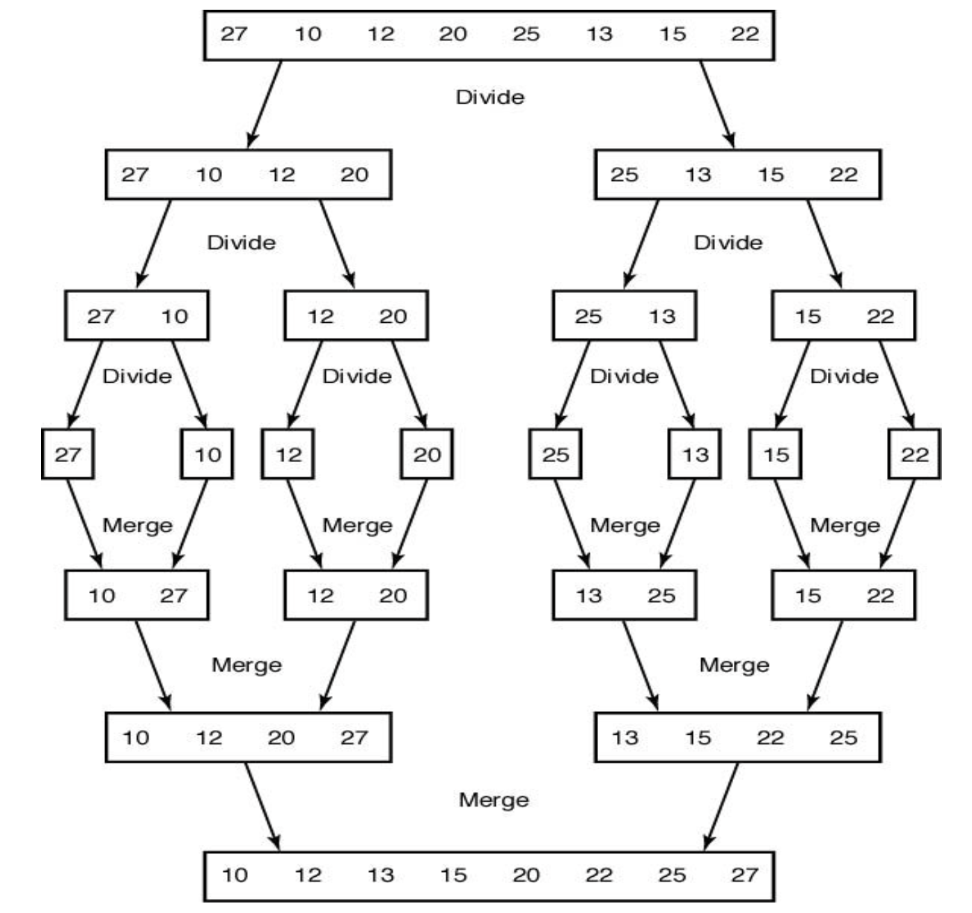
 void mergesort (int n, keytype S[]) {
    if (n > 1) {
const int h = n/2, m = n - h; keytype U[1..h], V[1..m];
          copy S[1] through S[h] to U[1] through U[h];
          copy S[h+1] through S[n] to V[1] through V[m];
          mergesort(h, U);
          mergesort(m, V);
          merge(h, m, U, V, S);
    }
}

각각 h와 m은 배열 U와 V의 크기이다.

Merge 알고리즘

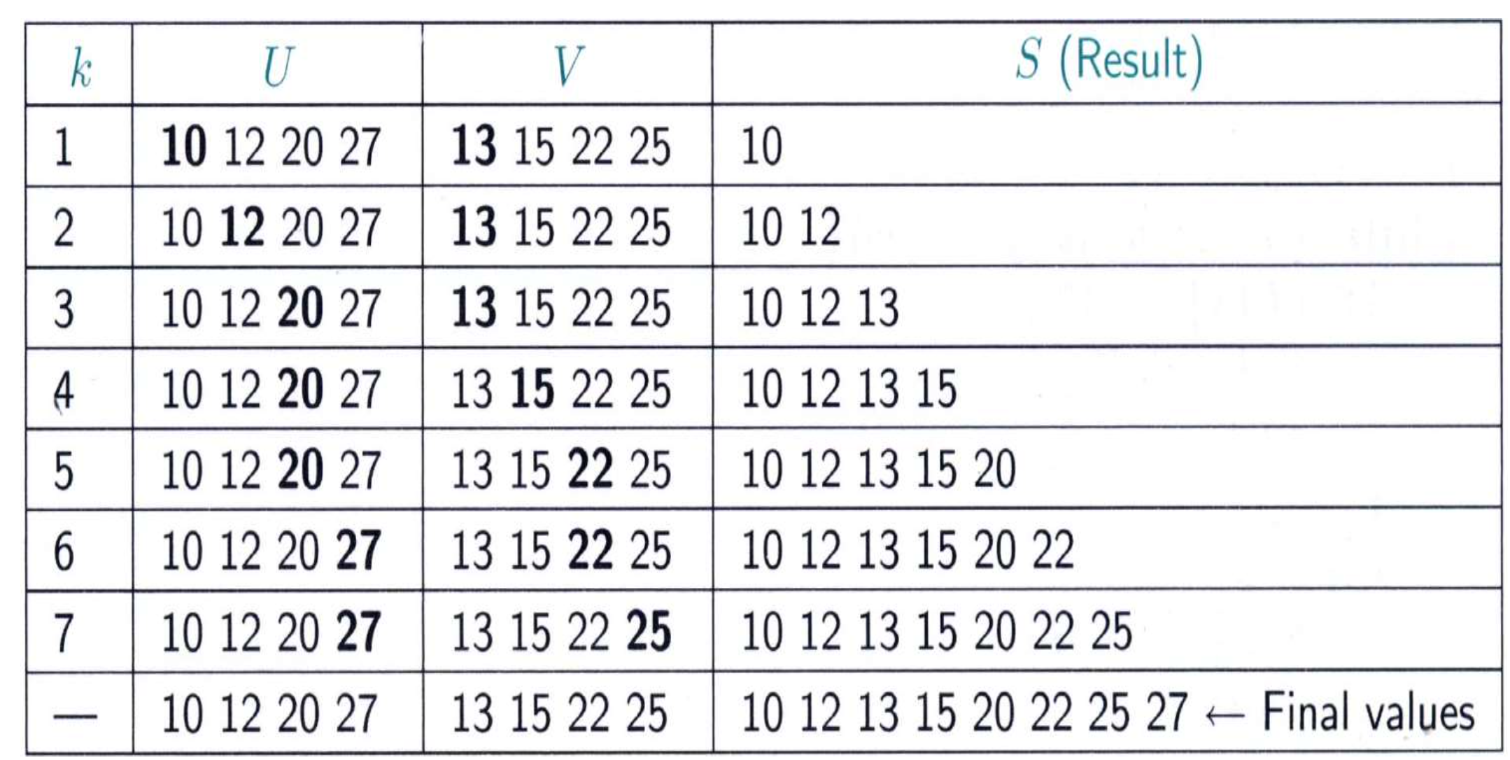
void merge(int h, int m, const keytype U[], const keytype V[],
           keytype S[]) {
index i, j, k;
i = 1; j = 1; k = 1;
while (i <= h && j <= m) {
      if (U[i] < V[j]) {
          S[k] = U[i];
i++; }
      else {
          S[k] = V[j];
j++; }
k++; }
  if (i > h)
      copy V[j] through V[m] to S[k] through S[h+m];
  else
      copy U[i] through U[h] to S[k] through S[h+m];
}

시간 복잡도 W(n) = n $lg$ n

⭐공간 복잡도가 향상된 Merge Sort(합병 정렬)

in-place sort (제자리정렬) 알고리즘

합병정렬 알고리즘은 제자리정렬 알고리즘이 아니다. 왜냐하면 입력인 배열 S이외에 U와 V를 추가로 만들어서 사용하기 때문이다.

void mergesort2 (index low, index high) { index mid;
if (low < high) {
mid = (low + high)/2; mergesort2(low, mid); mergesort2(mid+1, high); merge2(low, mid, high);
} }
...
...
mergesort2(1, n);

 void merge2(index low, index mid, index high) { index i, j, k;
keytype U[low..high];
i = low; j = mid + 1; k = low; while (i <= mid && j <= high) {
     if (S[i] < S[j]) {
         U[k] = S[i];
i++; }
     else {
         U[k] = S[j];
j++; }
k++; }
// 합병하는데 필요한 지역 배열
if (i > mid)
move S[j] through S[high] to U[k] through U[high];
else
move S[i] through S[mid] to U[k] through U[high];
move U[low] through U[high] to S[low] through S[high]; }

차이점: mergesort에서 기억공간을 사용하지 않음
U와 V를 사용하지 않기 때문에 공간복잡도가 2n -> n으로 줄어든다.

⭐Quick Sort

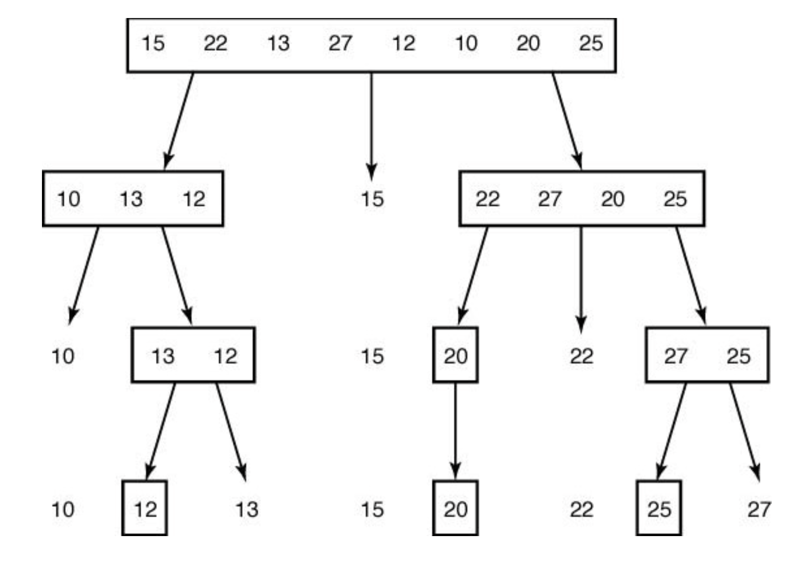
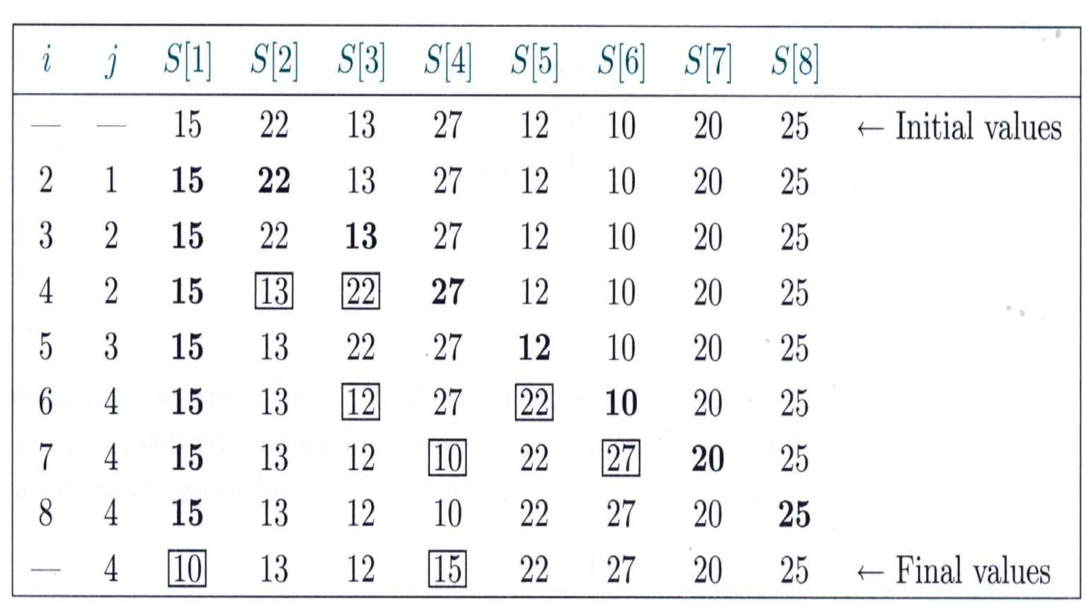
전략
i와 pivot을 비교해가며 pivot보다 작은 값들을 앞에 쌓아 pivot을 기준으로 앞에는 작은 값, 뒤에는 큰 값이 오도록 한다.

 void quicksort (index low, index high) {
    index pivotpoint;
    if (high > low) {
          partition(low, high, pivotpoint);
          quicksort(low, pivotpoint-1);
          quicksort(pivotpoint+1, high);
} }

 void partition (index low, index high, index& pivotpoint) {
     index i, j;
     keytype pivotitem;
pivotitem = S[low]; //pivotitem을 위한 첫번째 항목을 고른다 j = low;
for(i = low + 1; i <= high; i++)
         if (S[i] < pivotitem) {
            j++;
            exchange S[i] and S[j];
         }
     pivotpoint = j;
exchange S[low] and S[pivotpoint]; // pivotitem 값을 pivotpoint에 }

시간 복잡도
W(n) = $n^2$
A(n) = $nlgn$

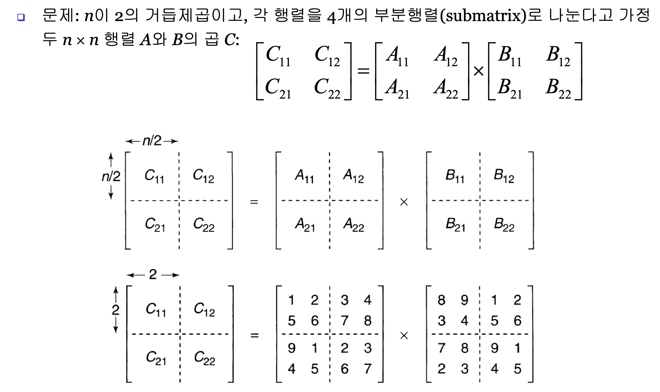
⭐Matrix Multiplication(행렬 곱셈)

순수하게 행렬 곱셈하는 방식으로 반복문으로 구현한다면?

 void matrixmult (int n, const number A[][],
                 const number B[][], number& C[][]) {
    index i, j, k;
    for (i = 1; i <= n; i++)
       for (j = 1; j <= n; j++) {
           C[i][j] = 0;
		} 
}

Every-case Time Complexity Analysis I:
basic Oper 1: 가장 안쪽의 루프에 있는 곱셈하는 연산
Every case:O( $n^3$ )

Every-case Time Complexity Analysis II:
basic Oper 2: 가장 안쪽의 루프에 있는 덧셈하는 연산
Every case:O( $n^3$ )

결국 시간 복잡도는 $n^3$

Divide-and-Conquer로 구현한 Matrix Multiplication

슈트라센 알고리즘

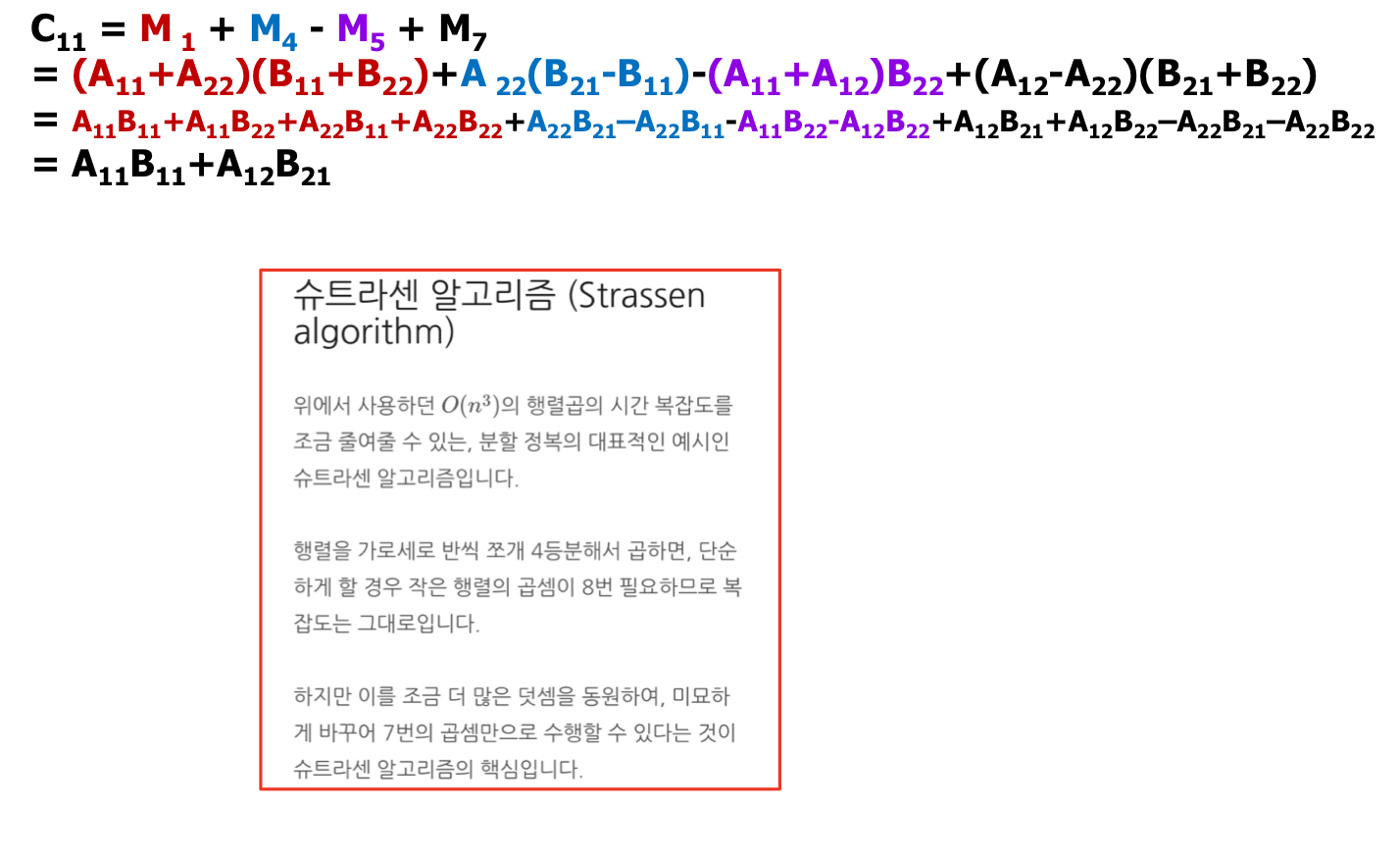
 void strassen (int n, n×n_matrix A, n×n_matrix B, n×n_matrix& C) { 
 	if (n <= threshold)
		compute C = A × B using the standard algorithm; 
	else {
		partition A into 4 submatrices A11, A12, A21, A22;
		partition B into 4 submatrices B11, B12, B21, B22;
		compute C = A × B using Strassen’s method;
		// example recursive call: strassen(n/2, A11+A22, B11+B22, M1)
	} 
}

basic Oper 1: 곱셈하는 연산
Every case:O( $n^{2.81}$ )

basic Oper 2: 가장 안쪽의 루프에 있는 덧셈하는 연산
Every case:O( $n^2$ )

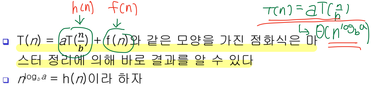
⭐마스터 정리

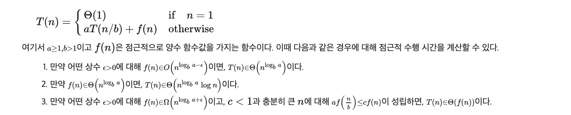
예시 문제)
T(n) = 8 * T( $n/4$ ) + $5n^2$
h(n) = $n^{log_48}$ = $n^{3/2}$
f(n) = $n^2$
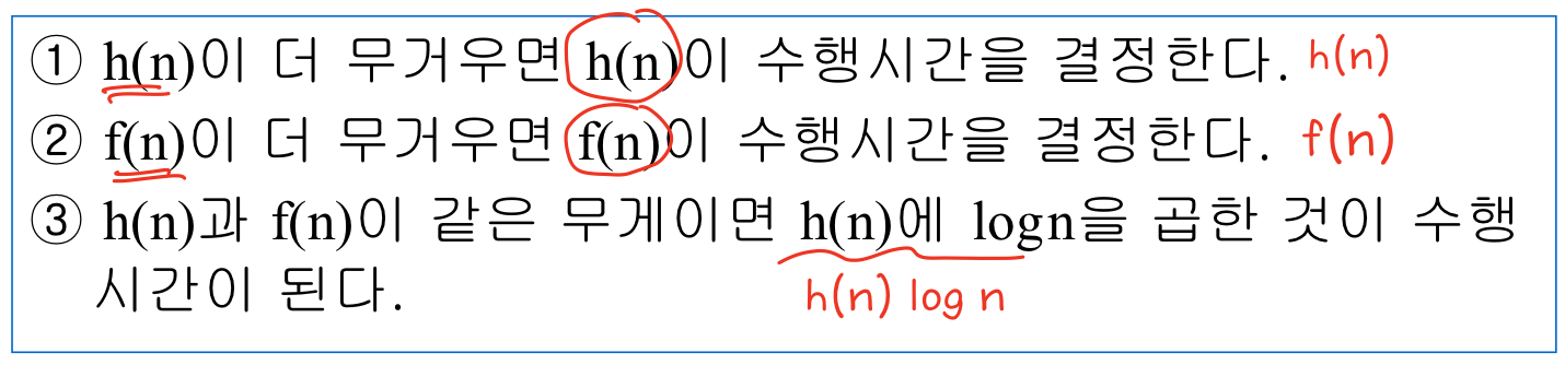
=> h(n)보다 f(n)이 더 무거우므로 f(n)이 수행시간을 결정한다.
그러므로 $n^2$ 이 시간복잡도 이다.