[ML] 실습 - 이직 여부 예측

• 선형 분류 모델의 학습 방법에 대해서 알 수 있다
• 가설 설정을 진행하여 직원의 이직 여부를 예측할 수 있다
• 분류평가지표에 대해서 알 수 있다

0. import library

import numpy as np
import pandas as pd
import matplotlib.pyplot as plt
import seaborn as sns

1. 문제 정의

• Role: HR 팀장
• 직원 이직 데이터를 분석하여 직원의 이직여부를 예측
• 이직과 연관있는 사람들의 특징을 파악하여 직원 관리 프로그램 개선
• 핵심인재 유출 방지

2. 데이터 수집

• IBM 가상 데이터 -> 직원 이직 여부 데이터

# 컬럼이 많은 경우 데이터 생략
# 그래서 전체 출력을 하고 싶은 경우에는, set_option 사용
pd.set_option('display.max_columns', None)
data = pd.read_csv('./data/job_transfer.csv')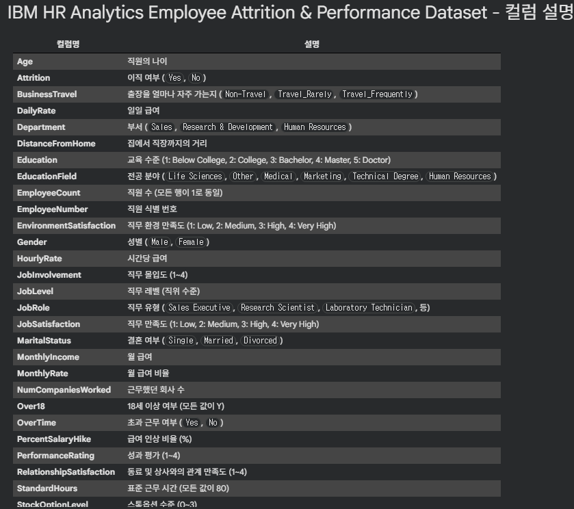
data.head()

• IBM HR Analytics Employee Attrition & Performance Dataset - 컬럼 설명

3. 데이터 전처리

• 결측치 없음

  data.isnull().sum().sort_values(ascending=False)

4. EDA

• 이직 컬럼 0/1로 변경 (추후, 이직률 계산하기 위함)

  # 이직 컬럼 0/1로 변경
  data['Attrition'] = np.where(data['Attrition']=='Yes',1,0)

• 이직률 = (이직한 직원수 / 전체 직원수) * 100

4.1. 연령대별 이직률 현황

1. 나이 데이터 범주화

   # 데이터 확인
   np.sort(data['Age'].unique())
   
   plt.figure(figsize=(5,3))
   plt.hist(data['Age'])
   plt.show()
   
   # 연속적인 데이터 범주화
   # 30세 미만, 30~40세, 40세 초과
   data['Age_gp'] = np.where(data['Age']<30, '30세 미만', np.where(data['Age']>40, '40세 초과', '30~40세'))

2. 연령대별 이직률 계산

   df_gp = data.groupby('Age_gp')['Attrition'].agg(['count','sum'])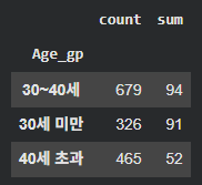

   

   df_gp['ratio'] = round(df_gp['sum'] / df_gp['count'] * 100, 1)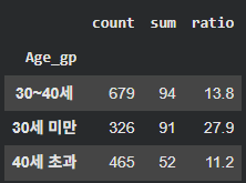

   

   나이가 어릴수록 이직률이 높다!

4.2. 성별에 따른 이직률

# 성별에 따른 이직률 현황
df_gp_gender = data.groupby('Gender')['Attrition'].agg(['count','sum'])
df_gp_gender['gender_ratio'] = round(df_gp_gender['sum'] / df_gp_gender['count'] * 100,1)

남자의 이직률이 더 높다

4.3. 성별/나이에 따른 이직률

df_gp_age_gender = data.groupby(['Gender', 'Age_gp'])['Attrition'].agg(['count','sum'])
df_gp_age_gender['ratio_gender_age'] = round(df_gp_age_gender['sum'] / df_gp_age_gender['count'] * 100, 1)

4.4. 가설을 세워 이직률이 높은 데이터를 낮게 만들자!

4.4.1. 가설1) 업무 만족도는 높으나 인간관계만족도가 떨어지면 이직한다

df_gp3 = data.groupby(['JobSatisfaction','RelationshipSatisfaction'])['Attrition'].agg(['count','sum'])
df_gp3 = round(df_gp3['sum'] / df_gp3['count'] * 100, 1)
df_gp3
# 업무 만족도가 낮은 직원은 인간관계가 나쁠수록 이직률이 증가한다
# 업무 만족도가 높은 직원은 인간관계에 영향을 받지 않음

→ 가설이 틀렸다!

4.4.2. 가설 2) 야근을 많이 하더라도 급여인상률이 높다면 이직률이 낮을 것이다

df_gp4 = data.groupby(['OverTime','PercentSalaryHike'])['Attrition'].agg(['count','sum'])
df_gp4 = round(df_gp4['sum'] / df_gp4['count'] * 100, 1)
df_gp4

4.4.3. 가설 3) 핵심 인재 중 집과의 거리가 멀면 이직률이 높을 것이다

1. 핵심 인재 범주화 (기준: 연봉인상률)

   1. 히스토그램으로 분포 확인

      plt.hist(data['PercentSalaryHike'])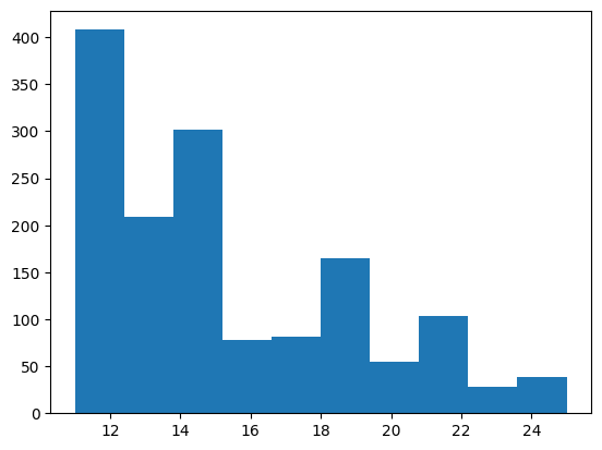

      

      <기준 설정> <15: Low / 16~19: Mid / >20: High

   2. 핵심 인력 범주 컬럼 추가

      data['Core'] = np.where(data['PercentSalaryHike']<16, 'Low', np.where(data['PercentSalaryHike']<20, 'Mid', 'High'))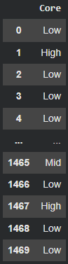

      

2. 거리 범주화

   1. 히스토그램으로 분포 확인

      plt.hist(data['DistanceFromHome'])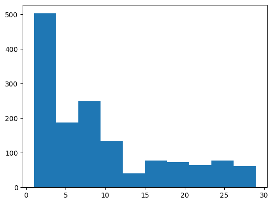

      

      <기준 설정> <10: near / ≥ 10: far

   b. 거리 범주화 기준 추가

   data['Dis'] = np.where(data['DistanceFromHome']<10, 'Near', 'far')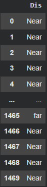

   

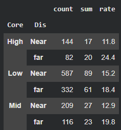
3. 계산

   df_gp5 = data.groupby(['Core','Dis'])['Attrition'].agg(['count','sum'])
   df_gp5['rate'] = round((df_gp5['sum']/df_gp5['count'])*100, 1)

   • 결론

     • 핵심 인력(연봉인상률 20% 이상) 중 집과 회사의 거리가 멀면 이직률이 높다.

     • 핵심 인력(연봉인상률 20% 이상) 중 집과 회사의 거리가 가까우면 이직률이 낮다.

     • 즉 , 핵심 인력 중 거리가 먼 직원에게 사택을 제공해 이직률을 감소시키자!

       

5. 모델링

5.1. 인코딩

1. Label Encoding: BusinessTravel 컬럼

   # 데이터 확인
   data['BusinessTravel'].unique()
   
   # 출장을 많이 갈수록 이직률이 높다
   
   # 방법 1) 수동 적용
   travel_type = ['Travel_Rarely', 'Travel_Frequently', 'Non-Travel']
   score = [0,1,2]
   dic_travel = dict(zip(travel_type, score))
   
   data['BusinessTravel'] = data['BusinessTravel'].map(dic_travel)
   data['BusinessTravel'].head()
   
   # 방법 2) sklearn 라이브러리 이용
   # from sklearn.preprocessing import LabelEncoding
   # le = LabelEncoding()
   # data['BusinessTravel'] = le.fit_transform(data['BusinessTravel'])

2. One-Hot Encoding: 나머지 컬럼 모두

   data_ondehot = pd.get_dummies(data)
   data_ondehot.head()

5.2. 데이터 분리

# X, target
X = data_ondehot.drop('Attrition', axis=1)
y = data_ondehot['Attrition']
X.shape, y.shape

# train, test
from sklearn.model_selection import train_test_split
X_train, X_test, y_train, y_test = train_test_split(X, y, train_size = 0.7, random_state=42, stratify=y)
X_train.shape, X_test.shape, y_train.shape, y_test.shape

5.3. Scaling

# scaling
from sklearn.preprocessing import StandardScaler
sc = StandardScaler()
numeric_list = [i for i in X_train.columns if X_train[i].dtype == 'int']
# numeric_list
X_train[numeric_list] = sc.fit_transform(X_train[numeric_list])
X_test[numeric_list] = sc.transform(X_test[numeric_list])

5.4. 모델 학습

# 선형분류모델 모델링
from sklearn.linear_model import LogisticRegression
from sklearn.svm import LinearSVC
from sklearn.metrics import accuracy_score

# Logistic
lg_model = LogisticRegression()
lg_model.fit(X_train, y_train)
pred_lg = lg_model.predict(X_test)
accu_lg = accuracy_score(y_test, pred_lg)
accu_lg

# SVM
svm_model = LinearSVC()
svm_model.fit(X_train, y_train)
pred_svm = svm_model.predict(X_test)
accu_svm = accuracy_score(y_test, pred_svm)
accu_svm

5.5. 예측 및 모델 평가

from sklearn.metrics import classification_report

# 1) Logistic Regerssion
print(classification_report(y_test, pred_lg))

# 결과
              precision    recall  f1-score   support

           0       0.89      0.97      0.93       370
           1       0.68      0.35      0.46        71

    accuracy                           0.87       441
   macro avg       0.78      0.66      0.69       441
weighted avg       0.85      0.87      0.85       441

# 해석

# 정확도는 높은 편이나, class 0과 class 1의 불균형이 확인됨
# 데이터의 클래스 불균형에서 오는 결과 -> 불균형 해결해줘야 함

# 2) Linear SVM
print(classification_report(y_test, pred_svm))

# 결과
              precision    recall  f1-score   support

           0       0.88      0.97      0.92       370
           1       0.68      0.32      0.44        71

    accuracy                           0.87       441
   macro avg       0.78      0.65      0.68       441
weighted avg       0.85      0.87      0.85       441

# 해석

# precision
# class 0 -> 모델이 0으로 예측한 것 중 0.88 가 실제 class 0
# class 1 -> 모델이 1  로 예측한 것 중 0.68 가 실제 class 1

# recall
# class 0 -> 실제 class 0 중에서 97%를 맞췄다
# class 1 -> 실제 class 1 중에서 44%를 맞췄다

# f1-score
# class 0 일대가 조화평균이 좋다, 균형있다.