
딥러닝 개요
- 딥러닝 (Deep Learning)
- 인공신경망을 기반으로 하는 머신러닝의 알고리즘 한 분야
- 비정형 대용량 데이터를 다루는데 많이 사용, 작은 데이터는 overfitting 가능성
- 정형 데이터 → table (표)
- 비정형 데이터 → 이미지(영상), 자연어, 음성
- 라이브러리
- Tensorflow
- 설치 :
pip install tensorflow→ cpu, gpu 포함 - cuda → GPU의 가상 명령어셋을 사용
- 설치 :
- Keras
- Tensorflow 2.0 부터 Keras가 텐서플로에 포함됨
- Tensorflow
MLP 구현
Keras 개발 Process
- 입력 텐서(X)와 출력 텐서(y)로 이뤄진 훈련 데이터를 정의
- 입력과 출력을 연결하는 Layer(층)으로 이뤄진 네트워크(모델)을 정의
- Sequential 방식, Functional API 방식, Subclass 방식
- 모델 Compile(컴파일)
- Training(학습/훈련)
MNIST 이미지 분류
- 흑백 손글씨 숫자 0-9까지 10개의 범주로 구분해놓은 데이터셋
- 28 * 28 pixel
- 60000개의 Train 이미지
- 10000개의 Test 이미지
1. 훈련 데이터 정의
-
import
import random import numpy as np import tensorflow as tf from tensorflow import keras # 설치된 tensorflow 버전 확인 print(tf.__version__) # seed값 설정 np.random.seed(0) # numpy tf.random.set_seed(0) # tensorflow random.seed(0) # random -
MNIST dataset Loading
-
keras 다운
(train_image, train_label), (test_image, test_label) = keras.datasets.mnist.load_data()→
-
shape 확인
train_image.shape, train_label.shape, test_image.shape, test_label.shape→
((60000, 28, 28), (60000,), (10000, 28, 28), (10000,))⇒ (60000 : 개수, (28,28) : 한 개 데이터의 shape)
⇒ 이미지 데이터 : 2차원 (gray scale) - (height, width)
, 3차원(color) - (height, width, channel-한 pixel 값을 구성하는 값들(R,G,B))
-
X값-image 확인
# X값-image 확인
import matplotlib.pyplot as plt
plt.figure(figsize=(10,5))

# 10개 이미지 출력
for i in range(10):
    plt.subplot(2, 5, i+1) # figure를 2X5으로 나눔, i+1 : 인덱스 구성
    plt.imshow(train_image[i], cmap='gray') # 최솟값 : black, 최대값 : white
    plt.title(f'{train_label[i]}', fontsize=20) # 정답 출력
    plt.axis('off') # spine(외각 경계선) 제거

plt.tight_layout() # subplot(axes)들 배치를 알아서 잘 해주는 것
plt.show()
→
-
-
데이터 전처리
X (Input Data Image)
- 0 ~ 1 사이의 값으로 정규화
- 타입을 float32로 변환
y (Output Data)
- one hot encoding 처리
tensorflow.keras.utils.to_categorical()
-
input image(X)를 정규화
- 2차원 - 0 : black, 255 : whilte ⇒ 차이가 많이 나니까 0~1 사이 값으로 바꾸겠다
dtype('uint8'): 부호 없이 8bit ⇒ unit 타입은 계산이 이상함 → float으로 변환
→train_image.min(), train_image.max(), train_image.dtype(0, 255, dtype('uint8'))X_train = train_image.astype("float32")/255 X_test = test_image.astype('float32')/255
- 2차원 - 0 : black, 255 : whilte ⇒ 차이가 많이 나니까 0~1 사이 값으로 바꾸겠다
-
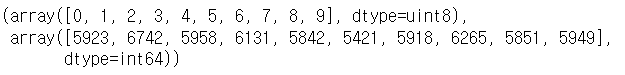
label(y)를 one hot encoding
np.unique(train_label, return_counts=True)→
# one hot encoding 처리하는 함수
y_train = keras.utils.to_categorical(train_label, num_classes=10) # num_classes=10 : 생략가능
y_test = keras.utils.to_categorical(test_label)

y_train.shape, y_test.shape
→
((60000, 10), (10000, 10))
2. 네트워크(모델) 정의
-
Sequential Model 정의 방법 2가지
- Sequential Model 정의 1: 모델객체를 생성하고 add() 메소드를 이용해 순서대로 Layer를 하나씩 추가
model = keras.Sequential() # 딥러닝 모델 생성 -> 빈모델을 생성 # Sequential Model에 layer추가 ## layer -> 함수. 이전 layer의 출력을 입력으로 받아서 처리한 뒤에 그 결과를 출력 model.add(keras.layers.InputLayer((28, 28))) # InputLayer: Input data의 shape 지정 model.add(keras.layers.Flatten()) # 다차원 입력을 1차원으로 변환 # unit/node/neuron 256개로 이루어진 layer를 생성 ## unit - 선형회귀 공식 1개. (X*W + b) model.add(keras.layers.Dense(units=256)) # 활성함수(Activation 함수)layer를 추가. ## RELU : max(x,0) => 비선형함수를 추가 model.add(keras.layers.ReLU()) model.add(keras.layers.Dense(units=128)) model.add(keras.layers.ReLU()) model.add(keras.layers.Dense(units=10)) # 출력(output) layer : 이 layer의 출력결과가 모델의 출력결과(예측결과) model.add(keras.layers.Softmax(name='output')) - Sequential Model 정의 2: 객체 생성시 Layer들을 순서대로 리스트로 묶어 전달
model2 = keras.Sequential([
    keras.layers.InputLayer((28,28)),
    keras.layers.Flatten(),
    keras.layers.Dense(256),
    keras.layers.ReLU(),
    keras.layers.Dense(units=128),
    keras.layers.ReLU(),
    keras.layers.Dense(10),
    keras.layers.Softmax()
])
- Sequential Model 정의 1: 모델객체를 생성하고 add() 메소드를 이용해 순서대로 Layer를 하나씩 추가
-
모델 구조 확인
model.summary() -
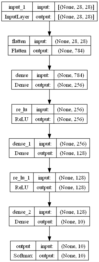
graphviz를 이용한 모델구조를 시각화
- (이미 설치해서) 업그레이드 버전 있으면 설치(-U) → restart
!pip install graphviz pydot pydotplus -U
keras.utils.plot_model(model,
show_shapes=True # input, output shape 같이 출력
, to_file='model_shapes.png' # 저장 파일명 지정 (생략 : model.png)
)→
- (이미 설치해서) 업그레이드 버전 있으면 설치(-U) → restart
3. 모델 Compile(컴파일)
- 정의된 모델을 학습할 수 있는 상태로 만들기
- Optimizer
- 손실함수
- 평가지표
model.compile(optimizer='adam', # 최적화 알고리즘 선택(필수)
            loss='categorical_crossentropy', # 손실함수 선택 (필수)
            metrics=['accuracy'] # 학습 도중/최종평가 때 출력되는 로그(학습기록)에 loss와 함께 같이 볼 추가 평가지표(선택)
            )
4. Training(학습/훈련)
-
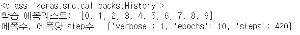
학습 (fit)
model.fit(): 학습과정의 Log를 History 객체에 넣어 반환- History : train 시 에폭별 평가지표값들을 모아서 제공
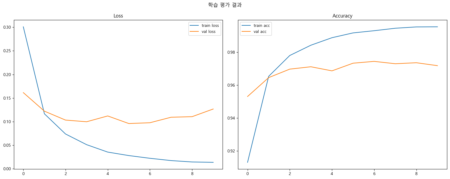
→history = model.fit(X_train, y_train, # Train dateset epochs=10, # train dataset을 몇 번 반복해서 학습할지 지정 batch_size=100, # 학습시 한번에 주입하는 데이터 개수, 지정한 개수 당 한번씩 파라미터 업데이트 한다. # 파라미터를 업데이트 하는 단위를 step이라고 함 validation_split=0.3 # 70% 학습, 30% 검증 데이터 # 생략하면 전체를 다 학습에 사용 )# 현재epoch/총epoch Epoch 10/10 # 현재step/총step (60000*0.7/100 = 420) |총학습시간| step당 걸린시간 420/420 [==============================] - 1s 3ms/step # trainset 검증결과 | val 검증결과 - loss: 0.0135 - accuracy: 0.9955 - val_loss: 0.1267 - val_accuracy: 0.9719 - 학습 에폭별 loss와 accuracy 변화량 시각화
-
테스트셋 평가
result = model.evaluate(X_test, y_test)→
313/313 [==============================] - 0s 1ms/step - loss: 0.1031 - accuracy: 0.9749
result→
[0.10311970114707947, 0.9749000072479248][loss, acc]
-
새로운 데이터 추론
-
predict()
- 분류: 각 클래스 별 확률 반환→ **class label 출력** - 이진 분류(binary classification) - `numpy.where(model.predict(x) > 0.5, 1, 0).astype("int32")` - 다중클래스 분류(multi-class classification) - `numpy.argmax(model.predict(x), axis=1)` - **회귀:** 최종 예측 결과X_new = X_test[:3] X_new.shape→
(3, 28, 28)
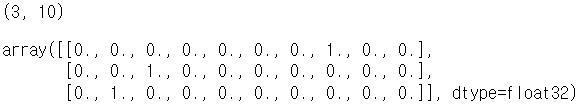
pred = model.predict(X_new)→
1/1 [==============================] - 0s 109ms/step
print(pred.shape)
np.round(pred, 3) # 반올림해서 보기
→

-
최대값 index 추출, 보통 마지막 축
np.argmax(pred, axis=1)
# np.argmax(y_test[:3], axis=-1)
→
array([7, 2, 1], dtype=int64)
5. 그림판 이미지로 확인
!pip install opencv-contrib-python
import cv2
# 이미지 읽어오기
two = cv2.imread("data/two.png", cv2.IMREAD_GRAYSCALE)
six = cv2.imread("data/six.png", cv2.IMREAD_GRAYSCALE)
print(type(two), type(six))
plt.imshow(six, cmap='gray')
-
plt.imshow(two, cmap='gray')=> 최종 결과
np.argmax(p, axis=1)→ array([2, 8], dtype=int64)
⇒ 하나 틀림