[논문리뷰] YOLO v1 리뷰 + 코드 구현(TensorFlow2)

안녕하세요. 밍기뉴와제제입니다.

오늘은 YOLO v1에 관한 리뷰를 하고 코드 구현한걸 설명해 드리고자 합니다. YOLO는 1-stage detector를 대표하는 모델 중 하나입니다. 현재 v5까지 나온걸로 압니다.

YOLO는 v1부터 v3까지는 주 저자가 Joseph Redmon, Ali Farhadi로 같지만 v4부터는 완전 다른 저자가 만들었다는 특이점이 있습니다. 허나 1-stage로 객체를 감지하는 모델, 처리 속도가 빠른 모델이라는 정신(?)은 공유하고 있습니다.

다시 본론으로 돌아갑시다. YOLO v1은 2015년에 나온 논문입니다. 매년 무수히 많은 논문이 나오는 딥러닝 분야에서는 엄청 오래된 논문이죠. 허나 1-stage detector 모델의 근본이라 할 수 있는 모델이기 때문에 한번은 보시고 구현해보는걸 추천드립니다. 논문 내용이 엄청 어려운 것도 아니고 구현 난이도도 Faster R-CNN같은 2-Stage detector에 비하면 매우 쉽기 때문에 금방 구현하실 수 있습니다.

그러면 먼저 YOLO에 대해 간단히 설명 드린 뒤 구현 코드를 설명해 드리도록 하겠습니다.

YOLO v1

---

전체적인 구조

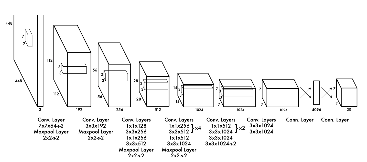
전체적인 구조는 다음과 같습니다. 448x448 크기의 이미지를 입력받아 여러층의 Layer를 거쳐 이미지에 있는 객체 위치와 객체의 정체를 알아내는 구조입니다. 한가지 모델로 object detection을 이뤄낸 것이죠. 그래서 1-Stage detector라고 하는겁니다.

Object Detection을 수행하는 모델은 크게 두가지 구조로 나뉩니다.

1. Backbone
2. Head

Backbone은 입력받은 이미지의 특성을 추출하는 역할을 하고 head에서는 특성이 추출된 특성 맵을 받아 object detection 역할을 수행합니다.

Backbone

보통 Backbone은 '특성 추출'이 목적이기 때문에 특성 추출에 최적화된 모델, 다시 말해 classification을 목적으로 만들어진 모델을 사용합니다. 왜냐하면 특성된 추출을 가지고 어떤 객체인지 알아내기 때문에 특성을 추출하는데 특화되었기 때문이죠. YOLO가 만들어지던 당시 가장 성능이 좋은 classification 모델은 VGG였습니다. 보통 VGG16을 썼죠.

허나 YOLO의 저자들은 VGG16을 쓰지 않고 자신들만의 Backbone을 만들었습니다. 바로 DarkNet이라는 모델입니다.

DarkNet의 특성은 입력받는 이미지의 해상도가 448x448로 VGG가 받던 224x224보다 4배나 더 크다는 것, 그리고 처리 속도가 빠르단 것이었습니다.

입력 해상도가 높은 이유는 Detection이 고해상도 이미지를 종종 요구하기 때문이었다고 논문에 나와있었고 처리 속도는 논문의 Experiment에 실험 결과가 나와있습니다.

참고로, 위 그림에서 DarkNet의 영역만 따로 추려내보면

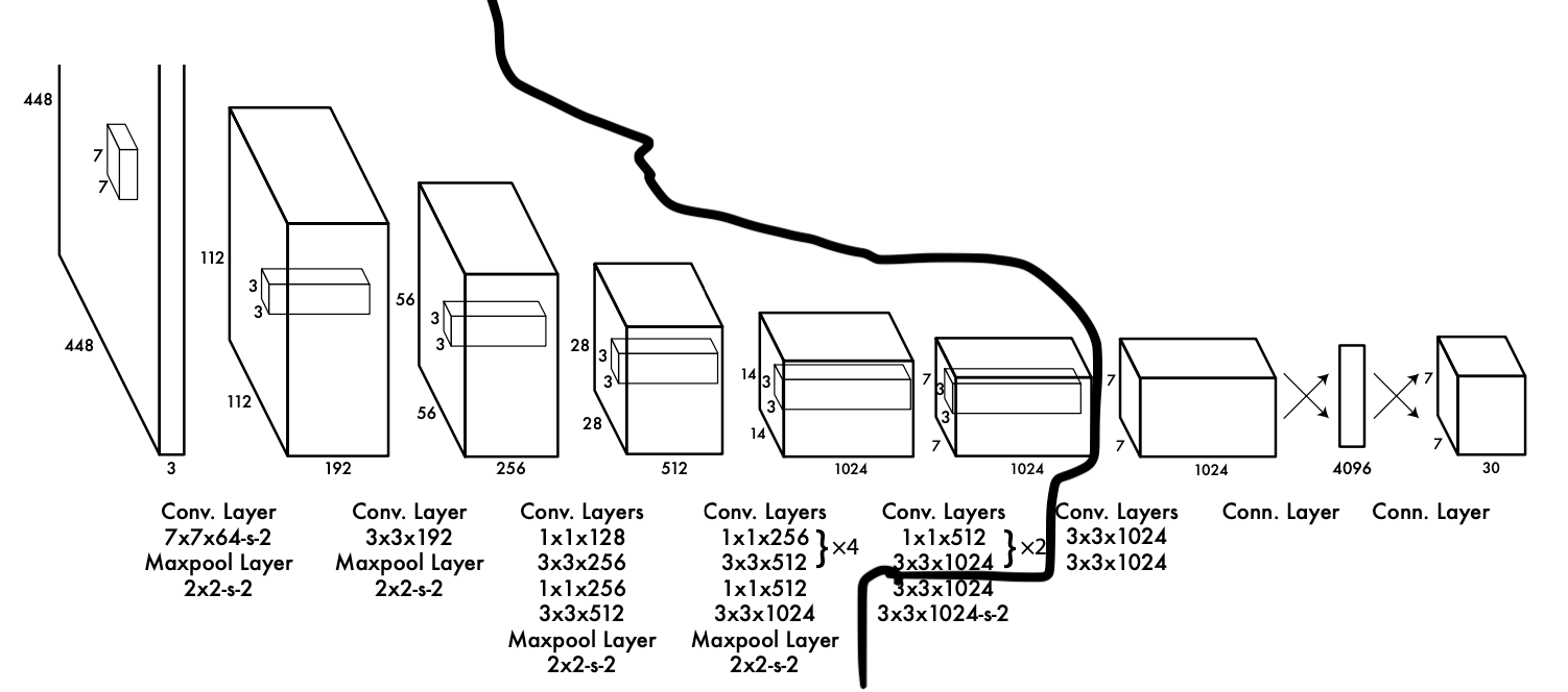
위와 같습니다. 왼쪽은 DarkNet, 오른쪽은 head입니다. head는 따로 이름이 지어지진 않았습니다.

그리고 추가로 설명드리자면 DarkNet은 CNN Layer 20층으로 구성되었고 Head는 CNN Layer 4층, FCN 2층으로 구성되었습니다.

Head

Head에 더 설명해 드리도록 하겠습니다. 여기서 주목할 부분은 마지막 출력값의 양식입니다. 448x448 해상도를 가진 이미지 한 장을 입력 받았을 때 7,7,30 사이즈의 3차원 텐서를 출력값으로 내놓습니다.

즉, 출력값의 셀 하나가 원본 이미지의 64x64영역을 대표하고 이 영역에서 검출된 30개의 데이터가 담겨있다는 뜻입니다. (448 / 7 = 64)

30개의 데이터는 다음과 같습니다.

1. 해당 영역을 중점으로 하는 객체의 Bounding Box 2개(x, y, w, h, confidence)
2. 해당 영역을 중점으로 하는 객체의 class score 20개

한 셀에서 2개의 bounding box를 검출하니까 총 검출되는 박스는 7x7x2 = 98개입니다. 이 98개의 박스는 각각 confidence를 가지고 있는데요, 말 그대로 신뢰도입니다. 이 bounding box를 얼마나 신뢰할 수 있느냐? 를 나타낸 점수라 보시면 됩니다.
수학적으로 나타내면 Pr(Object) * IoU입니다.

그리고 x, y는 해당 셀에 대해 normalize된 값이고 w,h는 전체 이미지에 대해 normalize된 값입니다. 예를 들어 (0,0)셀에서 나온 bounding box의 [x,y,w,h]가 [0.5, 0.5, 0.2, 0.2]면 변환했을 때 x = 31, y = 31, w = 448*0.2 = 96, h = 96이란 것이죠. (0,0) 셀은 원본 이미지의 (0,0)<->(63, 63)인 사각형을 대표하기 때문입니다.

20개의 class score는 해당 영역에서 검출된 객체가 어떤 클래스의 객체일 확률을 클래스 별로 나타낸 겁니다. 20은 이제 YOLO를 훈련시킬 때 사용할 PASCAL VOC 2007 dataset에 있는 클래스가 20종류라 20을 사용한 겁니다. 만약 다른 데이터셋을 사용한다면 20말고 다른 숫자를 사용할 수 있겠죠.

활성화 함수

저자는 활성화 함수도 다른걸 사용합니다. 저자는 Linear Activation function과

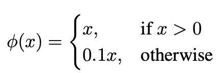
위와 같은 식을 가진 Leaky ReLU를 사용했습니다. Linear Activation function는 맨 마지막 Layer에 사용했는데요, 찾아보니 받은 값을 그대로 출력하는 함수였습니다. 음...그냥 사용하지 않았다! 와 동의어로 보시면 되겠습니다.
Leaky ReLU는 마지막 Layer를 제외한 모든 레이어에서 사용했습니다.

Loss function

손실 함수는 multi-task loss를 사용합니다.

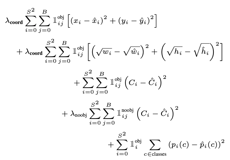
이렇게 생겼는데요, 위에 두줄은 bbox의 위치에 관한 손실(localization loss), 중간 3, 4 번째 줄은 confidence score에 관한 손실(confidence loss), 마지막 한 줄은 class score에 관한 에러입니다.(classification loss)

하나씩 뜯어보면 간단한 식들입니다. 여기 시그마에서 S^2는 전체 cell의 개수 = 49고 B는 각 셀에서 출력하는 bounding box의 개수 = 2입니다.

즉, localization loss, confidence loss는 해당 셀에 실제 객체의 중점이 있을 때 해당 셀에서 출력한 2개의 bounding box 중 Ground Truth Box와 IoU가 더높은 bounding box와 Ground Truth Box와의 loss를 계산한 것들입니다.

그리고 classification loss는 해당 셀에 실제 객체의 중점이 있을 때 해당 셀에서 얻은 class score와 label data 사이의 loss를 나타낸 값이죠.

후에 보여드릴 구현 코드를 보시면 더 쉽게 이해하실 수 있을겁니다.

Experiment : Backbone에 따른 성능 변화

저자는 Experiment 부분에서 Backbone에 따른 성능 변화를 나타냈습니다.

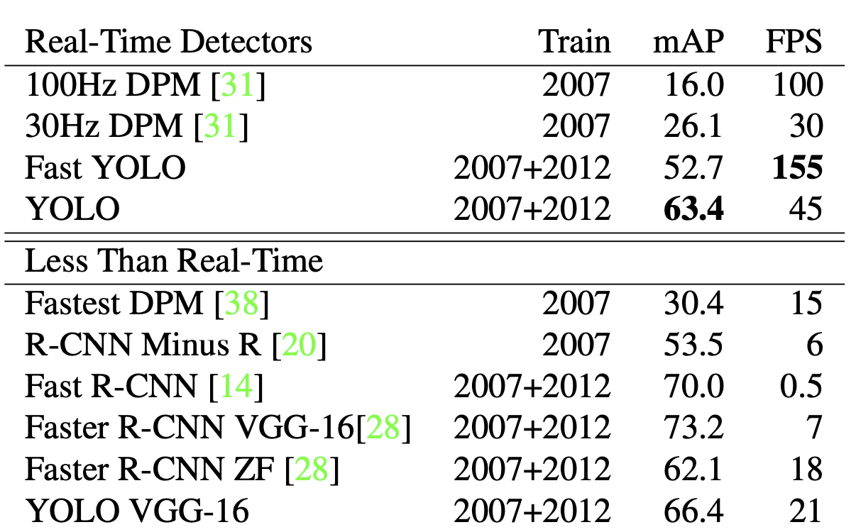
위 그림은 Detector들의 성능을 나타낸 겁니다. 여기서 YOLO가 성능, 처리속도를 같이 고려했을 때 가장 성능이 좋은 model로 나타난걸 알 수 있죠.

이 중 YOLO와 YOLO VGG-16이 보이실 겁니다. VGG-16은 backbone을 DarkNet대신 VGG-16을 사용한 모델인데요, 처리속도는 많이 떨어졌지만 정확도(mAP)는 좋아진 걸 확인하실 수 있습니다.

저는 원래 DarkNet이 있는 original YOLO를 구현하려고 했습니다. 그런데 텐서플로우2.x로 DarkNet이 구현 되어있는 걸 찾을 수가 없어 포기하고 VGG16으로 구현했습니다.

훈련

훈련 방법 등은 다음과 같습니다.

1. Backbone : ImageNet 2012 dataset으로 1주일간 훈련
2. Head : Weight decay = 0.0005, momentum = 0.9, batch size = 65, epoch = 135로 설정.
   처음에는 learning rate를 0.001로 맞춘 뒤 epoch = 75까지 0.01로 조금씩 상승시킴.
   그리고 이후 30회는 0.001로 훈련시키고 마지막 30회는 0.0001로 훈련시킴.
3. 데이터 증강(data augmentation) : 전체 이미지 사이즈의 20%만큼 random scaling을 합니다. 그리고 translation도 하며 원본 이미지의 1.5배만큼 HSV를 증가시킵니다.

논문 구현

---

이제 논문 구현에 대해 설명해 드리고자 합니다.

import

import numpy as np
import cv2
import xmltodict
from tqdm import tqdm
import tensorflow as tf
from glob import glob
from tensorflow.keras.callbacks import ModelCheckpoint

먼저 사용할 모듈들을 불러야죠. 여기서 따로 확인할 부분은

1. xmltodict : xml파일을 파이썬에서 사용
2. glob : 파일 경로 처리
3. cv2 : opencv 라이브러리

가 있겠습니다.

경로 불러오기

# 파일 경로
train_x_path = '파일경로'
train_y_path = '파일경로'

test_x_path = '파일경로'
test_y_path = '파일경로'

# 파일 경로 휙득
image_file_path_list = sorted([x for x in glob(train_x_path + '/**')])
xml_file_path_list = sorted([x for x in glob(train_y_path + '/**')])

test_image_file_path_list = sorted([x for x in glob(test_x_path + '/**')])
test_xml_file_path_list = sorted([x for x in glob(test_y_path + '/**')])

여기서는 데이터셋에 있는 사진(jpg), 라벨 데이터(xml)의 경로를 리스트에 담습니다.

예를 들면 image_file_path_list[0] = ".../000008.jpg"고 xml_file_path_list[0] = ".../000008.xml"와 같이 나타나죠.

데이터셋에 있는 클래스 종류 알아내기

def get_Classes_inImage(xml_file_list):
    Classes_inDataSet = []

    for xml_file_path in xml_file_list: 

        f = open(xml_file_path)
        xml_file = xmltodict.parse(f.read())
        # 사진에 객체가 여러개 있을 경우
        try: 
            for obj in xml_file['annotation']['object']:
                Classes_inDataSet.append(obj['name'].lower()) # 들어있는 객체 종류를 알아낸다
        # 사진에 객체가 하나만 있을 경우
        except TypeError as e: 
            Classes_inDataSet.append(xml_file['annotation']['object']['name'].lower()) 
        f.close()

    Classes_inDataSet = list(set(Classes_inDataSet))
    Classes_inDataSet.sort() # 알파벳 순으로 정렬

    return Classes_inDataSet

xml파일 리스트를 받아 YOLO를 훈련시킬 데이터셋에 있는 객체 종류를 알아냅니다.
xml파일에 여러개의 객체 정보가 있으면 try문 안에 있는 코드를 실행시키고 하나만 있으면 except문 안에 있는 코드를 실행시킵니다.

그렇게 데이터셋에 있는 모든 객체 정보를 얻습니다. 그러면 리스트는

['chair', 'chair', 'chair', 'chair', 'car', 'person', 'car',...]와 같이 나오겠죠? 여기서 중복된 문자열을 다 제거해야 데이터셋에 존재하는 객체의 종류가 얼마나 있는지 알 수 있을겁니다. 물론 각 객체가 뭔지도 알 수 있겠죠.

이를 위해 set으로 만들어줍니다. set은 중복되지 않은 원소가 들어있는 자료형이죠.
그러면 ['chair', 'car', 'person',...]이 들어있는 자료형을 얻고 편하게 사용하기 위해 리스트로 만들어줍니다.

그리고 sort를 해 알파벳 순으로 정리한 뒤 반환합니다.

Label data 처리

def get_label_fromImage(xml_file_path, Classes_inDataSet):

    f = open(xml_file_path)
    xml_file = xmltodict.parse(f.read()) 

    Image_Height = float(xml_file['annotation']['size']['height'])
    Image_Width  = float(xml_file['annotation']['size']['width'])

    label = np.zeros((7, 7, 25), dtype = float)
    
    try:
        for obj in xml_file['annotation']['object']:
            
            class_index = Classes_inDataSet.index(obj['name'].lower())
            
            # min, max좌표 얻기
            x_min = float(obj['bndbox']['xmin']) 
            y_min = float(obj['bndbox']['ymin'])
            x_max = float(obj['bndbox']['xmax']) 
            y_max = float(obj['bndbox']['ymax'])

            # 224*224에 맞게 변형시켜줌
            x_min = float((224.0/Image_Width)*x_min)
            y_min = float((224.0/Image_Height)*y_min)
            x_max = float((224.0/Image_Width)*x_max)
            y_max = float((224.0/Image_Height)*y_max)

            # 변형시킨걸 x,y,w,h로 만들기 
            x = (x_min + x_max)/2.0
            y = (y_min + y_max)/2.0
            w = x_max - x_min
            h = y_max - y_min

            # x,y가 속한 cell알아내기
            x_cell = int(x/32) # 0~6
            y_cell = int(y/32) # 0~6
            # cell의 중심 좌표는 (0.5, 0.5)다
            x_val_inCell = float((x - x_cell * 32.0)/32.0) # 0.0 ~ 1.0
            y_val_inCell = float((y - y_cell * 32.0)/32.0) # 0.0 ~ 1.0

            # w, h 를 0~1 사이의 값으로 만들기
            w = w / 224.0
            h = h / 224.0

            class_index_inCell = class_index + 5

            label[y_cell][x_cell][0] = x_val_inCell
            label[y_cell][x_cell][1] = y_val_inCell
            label[y_cell][x_cell][2] = w
            label[y_cell][x_cell][3] = h
            label[y_cell][x_cell][4] = 1.0
            label[y_cell][x_cell][class_index_inCell] = 1.0


    # single-object in image
    except TypeError as e : 
        # class의 index 휙득
        class_index = Classes_inDataSet.index(xml_file['annotation']['object']['name'].lower())
            
        # min, max좌표 얻기
        x_min = float(xml_file['annotation']['object']['bndbox']['xmin']) 
        y_min = float(xml_file['annotation']['object']['bndbox']['ymin'])
        x_max = float(xml_file['annotation']['object']['bndbox']['xmax']) 
        y_max = float(xml_file['annotation']['object']['bndbox']['ymax'])

        # 224*224에 맞게 변형시켜줌
        x_min = float((224.0/Image_Width)*x_min)
        y_min = float((224.0/Image_Height)*y_min)
        x_max = float((224.0/Image_Width)*x_max)
        y_max = float((224.0/Image_Height)*y_max)

        # 변형시킨걸 x,y,w,h로 만들기 
        x = (x_min + x_max)/2.0
        y = (y_min + y_max)/2.0
        w = x_max - x_min
        h = y_max - y_min

        # x,y가 속한 cell알아내기
        x_cell = int(x/32) # 0~6
        y_cell = int(y/32) # 0~6
        x_val_inCell = float((x - x_cell * 32.0)/32.0) # 0.0 ~ 1.0
        y_val_inCell = float((y - y_cell * 32.0)/32.0) # 0.0 ~ 1.0

        # w, h 를 0~1 사이의 값으로 만들기
        w = w / 224.0
        h = h / 224.0

        class_index_inCell = class_index + 5

        label[y_cell][x_cell][0] = x_val_inCell
        label[y_cell][x_cell][1] = y_val_inCell
        label[y_cell][x_cell][2] = w
        label[y_cell][x_cell][3] = h
        label[y_cell][x_cell][4] = 1.0
        label[y_cell][x_cell][class_index_inCell] = 1.0

    return label # np array로 반환

xml데이터를 사용할 수 있게 가공합니다.

출력값 양식이 [7, 7, 30]인데 label data는 객체당 하나의 bounding box가 있으니까 [7, 7, 25]로 만들었습니다.
자세한 처리과정은 코드를 보시는게 이해에 더 도움되실 거라 생각됩니다.

데이터셋을 사용할 수 있게 처리

def make_dataset(image_file_path_list, xml_file_path_list, Classes_inDataSet) :

    image_dataset = []
    label_dataset = []

    for i in tqdm(range(0, len(image_file_path_list)), desc = "make dataset"):
        image = cv2.imread(image_file_path_list[i]) 
        image = cv2.resize(image, (224, 224))/ 255.0 # 이미지를 넘파이 배열로 불러온 뒤 255로 나눠 픽셀별 R, G, B를 0~1사이의 값으로 만들어버린다.
        label = get_label_fromImage(xml_file_path_list[i], Classes_inDataSet)
        
        image_dataset.append(image)
        label_dataset.append(label)
    
    image_dataset = np.array(image_dataset, dtype="object")
    label_dataset = np.array(label_dataset, dtype="object")
    
    image_dataset = np.reshape(image_dataset, (-1, 224, 224, 3)).astype(np.float32)
    label_dataset = np.reshape(label_dataset, (-1, 7, 7, 25))

    return image_dataset, tf.convert_to_tensor(label_dataset, dtype=tf.float32)

데이터셋을 만듭니다. 앞서 말씀드린 get_label_fromImage()와 opencv에 있는 이미지 처리 함수를 사용해 넘파이 형식의 데이터셋을 생성합니다.
여기서 데이터 증강을 구현해야 했는데요, 저는 데이터 증강을 구현하지 않았습니다. 왜냐하면 어떻게 해야할지 감을 못잡았기 때문입니다. 전체 데이터 대비 얼마나 데이터 증강으로 데이터를 증가시켜야할지도 감이 안잡혔고 이미지를 변환시키면 이에 맞춰 label data도 변환시켜줬어야 했는데 그 과정이 너무 번거로웠습니다. 그래서 하지 않았습니다.

Pre-trained model 가져오기(Backbone)

max_num = len(tf.keras.applications.VGG16(weights='imagenet', include_top=False,  input_shape=(224, 224, 3)).layers) # 레이어 최대 개수

YOLO = tf.keras.models.Sequential(name = "YOLO")
for i in range(0, max_num-1):
    YOLO.add(tf.keras.applications.VGG16(weights='imagenet', include_top=False,  input_shape=(224, 224, 3)).layers[i])

initializer = tf.keras.initializers.RandomNormal(mean=0.0, stddev=0.01, seed=None)
leaky_relu = tf.keras.layers.LeakyReLU(alpha=0.01)  
regularizer = tf.keras.regularizers.l2(0.0005) # L2 규제 == weight decay.

for layer in YOLO.layers:
    # 훈련 X
    layer.trainable=False
    if (hasattr(layer,'activation'))==True:
        layer.activation = leaky_relu
        

사전 훈련된 VGG16을 가져옵니다. Tensorflow는 backbone으로 사용하는 대표적인 모델들을 자신들의 model class로 제공하고 있습니다.
제가 이걸 만들 때 쯤에는 VGG가 제일 좋은 model이었는데 최근에 업데이트를 했더라고요.

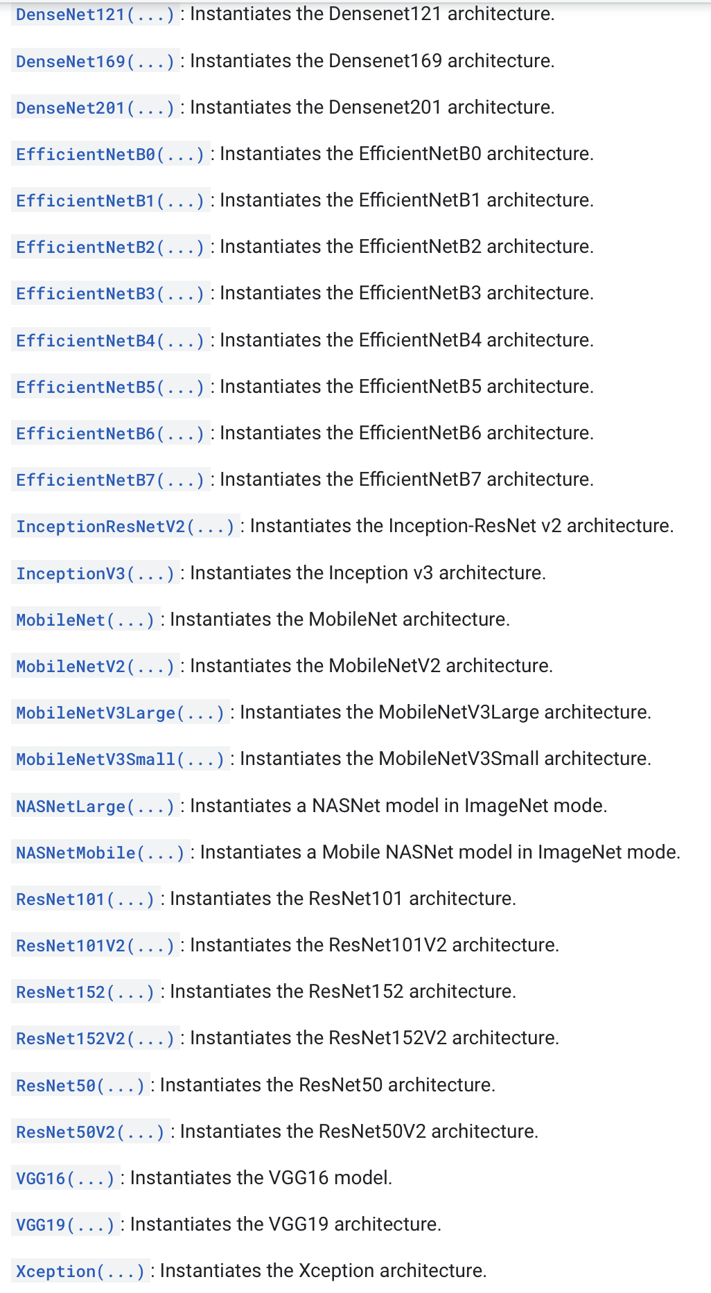
엄청 많이 추가되었습니다. 요즘 논문에서도 Backbone으로 많이 쓰는 ResNet과 ResNet보다 이후에 나온 DenseNet 등 많은 모델이 추가되어 모델 설계하기 더 좋아졌습니다. 굳굳.

Head 설계

YOLO.add(tf.keras.layers.Conv2D(1024, (3, 3), activation=leaky_relu, kernel_initializer=initializer, kernel_regularizer = regularizer, padding = 'SAME', name = "detection_conv1", dtype='float32'))
YOLO.add(tf.keras.layers.Conv2D(1024, (3, 3), activation=leaky_relu, kernel_initializer=initializer, kernel_regularizer = regularizer, padding = 'SAME', name = "detection_conv2", dtype='float32'))
YOLO.add(tf.keras.layers.MaxPool2D((2, 2)))
YOLO.add(tf.keras.layers.Conv2D(1024, (3, 3), activation=leaky_relu, kernel_initializer=initializer, kernel_regularizer = regularizer, padding = 'SAME', name = "detection_conv3", dtype='float32'))
YOLO.add(tf.keras.layers.Conv2D(1024, (3, 3), activation=leaky_relu, kernel_initializer=initializer, kernel_regularizer = regularizer, padding = 'SAME', name = "detection_conv4", dtype='float32'))
# Linear 부분
YOLO.add(tf.keras.layers.Flatten())
YOLO.add(tf.keras.layers.Dense(4096, activation=leaky_relu, kernel_initializer = initializer, kernel_regularizer = regularizer, name = "detection_linear1", dtype='float32'))
YOLO.add(tf.keras.layers.Dropout(.5))
# 마지막 레이어의 활성화 함수는 선형 활성화 함수인데 이건 입력값을 그대로 내보내는거라 activation을 따로 지정하지 않았다.
YOLO.add(tf.keras.layers.Dense(1470, kernel_initializer = initializer, kernel_regularizer = regularizer, name = "detection_linear2", dtype='float32')) 
YOLO.add(tf.keras.layers.Reshape((7, 7, 30), name = 'output', dtype='float32'))

Backbone으로 추출된 특성 맵을 입력값으로 받아 object detection을 수행하는 Head입니다.
[7,7,30] 사이즈의 텐서를 출력하는 마지막 레이어 YOLO.add(tf.keras.layers.Dense(1470, ...)) 는 활성화 함수를 지정하지 않습니다. 왜냐하면 linear activation function을 사용하라고 했는데 이게 출력값을 그대로 내보내는 방식이기 때문입니다.

그리고 왜 출력값의 사이즈가 1470이냐면 7730 = 1470이라서 그렇습니다. 그리고 이대로 내보내면 7,7,30 형태가 아니기 때문에 맨 마지막에 ReShape 레이어를 추가해줍니다.

Loss Function

def yolo_multitask_loss(y_true, y_pred): # 커스텀 손실함수. 배치 단위로 값이 들어온다
    
    # YOLOv1의 Loss function은 3개로 나뉜다. localization, confidence, classification
    # localization은 추측한 box랑 ground truth box의 오차
    
    batch_loss = 0
    count = len(y_true)
    for i in range(0, len(y_true)) :
        y_true_unit = tf.identity(y_true[i])
        y_pred_unit = tf.identity(y_pred[i])
        
        y_true_unit = tf.reshape(y_true_unit, [49, 25])
        y_pred_unit = tf.reshape(y_pred_unit, [49, 30])
        
        loss = 0
        
        for j in range(0, len(y_true_unit)) :
            # pred = [1, 30], true = [1, 25]
            
            bbox1_pred = tf.identity(y_pred_unit[j][:4])
            bbox1_pred_confidence = tf.identity(y_pred_unit[j][4])
            bbox2_pred = tf.identity(y_pred_unit[j][5:9])
            bbox2_pred_confidence = tf.identity(y_pred_unit[j][9])
            class_pred = tf.identity(y_pred_unit[j][10:])
            
            bbox_true = tf.identity(y_true_unit[j][:4])
            bbox_true_confidence = tf.identity(y_true_unit[j][4])
            class_true = tf.identity(y_true_unit[j][5:])
            
            # IoU 구하기
            # x,y,w,h -> min_x, min_y, max_x, max_y로 변환
            box_pred_1_np = bbox1_pred.numpy()
            box_pred_2_np = bbox2_pred.numpy()
            box_true_np   = bbox_true.numpy()

            box_pred_1_area = box_pred_1_np[2] * box_pred_1_np[3]
            box_pred_2_area = box_pred_2_np[2] * box_pred_2_np[3]
            box_true_area   = box_true_np[2]  * box_true_np[3]

            box_pred_1_minmax = np.asarray([box_pred_1_np[0] - 0.5*box_pred_1_np[2], box_pred_1_np[1] - 0.5*box_pred_1_np[3], box_pred_1_np[0] + 0.5*box_pred_1_np[2], box_pred_1_np[1] + 0.5*box_pred_1_np[3]])
            box_pred_2_minmax = np.asarray([box_pred_2_np[0] - 0.5*box_pred_2_np[2], box_pred_2_np[1] - 0.5*box_pred_2_np[3], box_pred_2_np[0] + 0.5*box_pred_2_np[2], box_pred_2_np[1] + 0.5*box_pred_2_np[3]])
            box_true_minmax   = np.asarray([box_true_np[0] - 0.5*box_true_np[2], box_true_np[1] - 0.5*box_true_np[3], box_true_np[0] + 0.5*box_true_np[2], box_true_np[1] + 0.5*box_true_np[3]])

            # 곂치는 영역의 (min_x, min_y, max_x, max_y)
            InterSection_pred_1_with_true = [max(box_pred_1_minmax[0], box_true_minmax[0]), max(box_pred_1_minmax[1], box_true_minmax[1]), min(box_pred_1_minmax[2], box_true_minmax[2]), min(box_pred_1_minmax[3], box_true_minmax[3])]
            InterSection_pred_2_with_true = [max(box_pred_2_minmax[0], box_true_minmax[0]), max(box_pred_2_minmax[1], box_true_minmax[1]), min(box_pred_2_minmax[2], box_true_minmax[2]), min(box_pred_2_minmax[3], box_true_minmax[3])]

            # 박스별로 IoU를 구한다
            IntersectionArea_pred_1_true = 0

            # 음수 * 음수 = 양수일 수도 있으니 검사를 한다.
            if (InterSection_pred_1_with_true[2] - InterSection_pred_1_with_true[0] + 1) >= 0 and (InterSection_pred_1_with_true[3] - InterSection_pred_1_with_true[1] + 1) >= 0 :
                    IntersectionArea_pred_1_true = (InterSection_pred_1_with_true[2] - InterSection_pred_1_with_true[0] + 1) * InterSection_pred_1_with_true[3] - InterSection_pred_1_with_true[1] + 1

            IntersectionArea_pred_2_true = 0

            if (InterSection_pred_2_with_true[2] - InterSection_pred_2_with_true[0] + 1) >= 0 and (InterSection_pred_2_with_true[3] - InterSection_pred_2_with_true[1] + 1) >= 0 :
                    IntersectionArea_pred_2_true = (InterSection_pred_2_with_true[2] - InterSection_pred_2_with_true[0] + 1) * InterSection_pred_2_with_true[3] - InterSection_pred_2_with_true[1] + 1

            Union_pred_1_true = box_pred_1_area + box_true_area - IntersectionArea_pred_1_true
            Union_pred_2_true = box_pred_2_area + box_true_area - IntersectionArea_pred_2_true

            IoU_box_1 = IntersectionArea_pred_1_true/Union_pred_1_true
            IoU_box_2 = IntersectionArea_pred_2_true/Union_pred_2_true
                        
            responsible_IoU = 0
            responsible_box = 0
            responsible_bbox_confidence = 0
            non_responsible_bbox_confidence = 0

            # box1, box2 중 responsible한걸 선택(IoU 기준)
            if IoU_box_1 >= IoU_box_2 :
                responsible_IoU = IoU_box_1
                responsible_box = tf.identity(bbox1_pred)
                responsible_bbox_confidence = tf.identity(bbox1_pred_confidence)
                non_responsible_bbox_confidence = tf.identity(bbox2_pred_confidence)
                                
            else :
                responsible_IoU = IoU_box_2
                responsible_box = tf.identity(bbox2_pred)
                responsible_bbox_confidence = tf.identity(bbox2_pred_confidence)
                non_responsible_bbox_confidence = tf.identity(bbox1_pred_confidence)
                
            # 1obj(i) 정하기(해당 셀에 객체의 중심좌표가 들어있는가?)
            obj_exist = tf.ones_like(bbox_true_confidence)
            if box_true_np[0] == 0.0 and box_true_np[1] == 0.0 and box_true_np[2] == 0.0 and box_true_np[3] == 0.0 : 
                obj_exist = tf.zeros_like(bbox_true_confidence) 
            
                        
            # 만약 해당 cell에 객체가 없으면 confidence error의 no object 파트만 판단. (label된 값에서 알아서 해결)
            # 0~3 : bbox1의 위치 정보, 4 : bbox1의 bbox confidence score, 5~8 : bbox2의 위치 정보, 9 : bbox2의 confidence score, 10~29 : cell에 존재하는 클래스 확률 = pr(class | object) 

            # localization error 구하기(x,y,w,h). x, y는 해당 grid cell의 중심 좌표와 offset이고 w, h는 전체 이미지에 대해 정규화된 값이다. 즉, 범위가 0~1이다.
            localization_err_x = tf.math.pow( tf.math.subtract(bbox_true[0], responsible_box[0]), 2) # (x-x_hat)^2
            localization_err_y = tf.math.pow( tf.math.subtract(bbox_true[1], responsible_box[1]), 2) # (y-y_hat)^2

            localization_err_w = tf.math.pow( tf.math.subtract(tf.sqrt(bbox_true[2]), tf.sqrt(responsible_box[2])), 2) # (sqrt(w) - sqrt(w_hat))^2
            localization_err_h = tf.math.pow( tf.math.subtract(tf.sqrt(bbox_true[3]), tf.sqrt(responsible_box[3])), 2) # (sqrt(h) - sqrt(h_hat))^2
            
            # nan 방지
            if tf.math.is_nan(localization_err_w).numpy() == True :
                localization_err_w = tf.zeros_like(localization_err_w, dtype=tf.float32)
            
            if tf.math.is_nan(localization_err_h).numpy() == True :
                localization_err_h = tf.zeros_like(localization_err_h, dtype=tf.float32)
            
            localization_err_1 = tf.math.add(localization_err_x, localization_err_y)
            localization_err_2 = tf.math.add(localization_err_w, localization_err_h)
            localization_err = tf.math.add(localization_err_1, localization_err_2)
            
            weighted_localization_err = tf.math.multiply(localization_err, 5.0) # 5.0 : λ_coord
            weighted_localization_err = tf.math.multiply(weighted_localization_err, obj_exist) # 1obj(i) 곱하기
            
            # confidence error 구하기. true의 경우 답인 객체는 1 * ()고 아니면 0*()가 된다. 
            # index 4, 9에 있는 값(0~1)이 해당 박스에 객체가 있을 확률을 나타낸거다. Pr(obj in bbox)
            
            class_confidence_score_obj = tf.math.pow(tf.math.subtract(responsible_bbox_confidence, bbox_true_confidence), 2)
            class_confidence_score_noobj = tf.math.pow(tf.math.subtract(non_responsible_bbox_confidence, tf.zeros_like(bbox_true_confidence)), 2)
            class_confidence_score_noobj = tf.math.multiply(class_confidence_score_noobj, 0.5)
            
            class_confidence_score_obj = tf.math.multiply(class_confidence_score_obj, obj_exist)
            class_confidence_score_noobj = tf.math.multiply(class_confidence_score_noobj, tf.math.subtract(tf.ones_like(obj_exist), obj_exist)) # 객체가 존재하면 0, 존재하지 않으면 1을 곱합
            
            class_confidence_score = tf.math.add(class_confidence_score_obj,  class_confidence_score_noobj) 
            
            # classification loss(10~29. 인덱스 10~29에 해당되는 값은 Pr(Classi |Object)이다. 객체가 cell안에 있을 때 해당 객체일 확률
            # class_true_oneCell는 진짜 객체는 1이고 나머지는 0일거다. 
            
            tf.math.pow(tf.math.subtract(class_true, class_pred), 2.0) # 여기서 에러
            
            classification_err = tf.math.pow(tf.math.subtract(class_true, class_pred), 2.0)
            classification_err = tf.math.reduce_sum(classification_err)
            classification_err = tf.math.multiply(classification_err, obj_exist)

            # loss합체
            loss_OneCell_1 = tf.math.add(weighted_localization_err, class_confidence_score)
            loss_OneCell = tf.math.add(loss_OneCell_1, classification_err)
            
            if loss == 0 :
                loss = tf.identity(loss_OneCell)
            else :
                loss = tf.math.add(loss, loss_OneCell)
        
        if batch_loss == 0 :
            batch_loss = tf.identity(loss)
        else :
            batch_loss = tf.math.add(batch_loss, loss)
        
    # 배치에 대한 loss 구하기
    count = tf.Variable(float(count))
    batch_loss = tf.math.divide(batch_loss, count)
    
    return batch_loss

모델 설계에서 제일 공들인 부분입니다. 미니배치 단위(64)로 입력 데이터가 들어오고 출력데이터가 나오기 때문에 [7,7,30] 사이즈씩 뽑아서 loss를 계산합니다.

그리고 [7,7,30]을 [49,30]으로 변경 후 [1,30] 사이즈를 가진 텐서별로 loss를 구합니다. 이 때 인덱스 0~4는 bounding box1, 5~9는 bounding box2, 10~29는 class score이며 해당 셀에 객체의 중심이 있을 경우 예측한 bounding box 중 IoU가 높은 Bounding box와의 localization loss, confidence loss를 구하고 class score도 구해줍니다.

아마 코드를 보시면 더 자세히 이해하실 수 있지 않을까 싶습니다.

훈련 세팅

BATCH_SIZE = 64
EPOCH = 135

# "We continue training with 10−2 for 75 epochs, then 10−3 for 30 epochs, and finally 10−4 for 30 epochs" 구현
def lr_schedule(epoch, lr): # epoch는 0부터 시작
    if epoch >=0 and epoch < 75 :
        lr = 0.001 + 0.009 * (float(epoch)/(75.0)) # 가중치를 0.001 ~ 0.0075로 변경
        return lr
    elif epoch >= 75 and epoch < 105 :
        lr = 0.001
        return lr
    else : 
        lr = 0.0001
        return lr

# loss 제일 낮을 때 가중치 저장
filename = 'yolo.h5'

checkpoint = ModelCheckpoint(filename,             # file명을 지정합니다
                             verbose=1,            # 로그를 출력합니다
                             save_best_only=True   # 가장 best 값만 저장합니다
                            )
                            
optimizer = tf.keras.optimizers.SGD(learning_rate=0.001, momentum = 0.9)

YOLO.compile(loss = yolo_multitask_loss, optimizer=optimizer, run_eagerly=True)

여기서는 훈련을 위한 세팅을 합니다. minibatch의 크기는 얼마고 epoch는 얼마고...이런걸 세팅하는 부분입니다.

그리고 lr_schedule라는 함수가 있는데요, 이는 한 epoch를 끝낸 뒤 호출되는 함수입니다. epoch와 learning rate를 받아 현재 epoch를 기준으로 learning rate를 조정합니다.

그리고 checkpoint = ModelCheckpoint() 역시 한 epoch를 끝낸 뒤 호출되는 함수입니다. 얘는 이전 epoch에서 달성했던 성능과 비교 후 개선되었으면 가중치를 저장합니다. 이 때 개선의 기준을 측정하는 수치로는 loss, validation loss, accuracy, validation accuracy 등 다양합니다.

그리고 gradient를 받고 가중치를 조정할 optimizer를 sgd로 설정합니다. 이 때 momentum도 같이 설정했습니다.

마지막으로 compile()에서 YOLO를 훈련시킬 때 적용할 방법(loss구하는 법, 구한 loss로 가중치 조정하는 방법)을 설정합니다. run_eagerly=True는 loss함수를 발동시킬 때 Tensor를 numpy array로 변환시키는 걸 허용해준다는 뜻입니다. 기본값은 False라 훈련 과정에서 호출하는 함수 내에서는 Tensor를 numpy array로 변경할 수 없습니다.

훈련

YOLO.fit(train_image_dataset, train_label_dataset,
          batch_size=BATCH_SIZE,
          validation_data = (val_image_dataset, val_label_dataset),
          epochs=EPOCH,
          verbose=1,
          callbacks=[checkpoint, tf.keras.callbacks.LearningRateScheduler(lr_schedule)])

모델을 훈련시킵니다. 훈련용 데이터셋, 검증용 데이터셋, epoch, 매 epoch마다 호출시킬 함수들 등을 지정합니다.

테스트

---

이렇게 모델을 훈련시켰으면 테스트를 해봐야죠. 테스트 함수는 다음과 같습니다.

# 출력된 bbox 정보를 사진에 출력할 수 있게 처리
def process_bbox(x, y, bbox, image_size, classes_score, Classes_inDataSet) : 
    # size 처리
    bbox_x = ((32.0 * x) + (bbox[0] * 32.0)) * (image_size[0]/224.0) # 예를 들어 x = 0이면 0~32사이에 중점의 x좌표가 존재
    bbox_y = ((32.0 * y) + (bbox[1] * 32.0)) * (image_size[1]/224.0) # 예를 들어 x = 0이면 0~32사이에 중점의 x좌표가 존재
    bbox_w = bbox[2] * image_size[0] # 전체 이미지 대비 백분위
    bbox_h = bbox[3] * image_size[1] # 전체 이미지 대비 백분위
    
    min_x = int(bbox_x - bbox_w/2)
    min_y = int(bbox_y - bbox_h/2)
    max_x = int(bbox_x + bbox_w/2)
    max_y = int(bbox_y + bbox_h/2)
    
    idx_class_highest_score = np.argmax(classes_score)
    class_highest_score = classes_score[idx_class_highest_score] # 가장 높은 class score
    class_highest_score_name = Classes_inDataSet[idx_class_highest_score] # 가장 높은 score를 가진 class의 이름
    
    output_bbox = [min_x, min_y, max_x, max_y, class_highest_score, class_highest_score_name]

    return output_bbox # [x, y, w, h, class_highest_score, class_highest_score_name]로 구성된 list출력
    
def nms(bbox_list) : 
    nms_bbox_list = []
    for i in range(0, len(bbox_list)) :
        
        if bbox_list[i][4] > 0.5 : # class score가 0.5넘기는 것만 출력하기
            nms_bbox_list.append(bbox_list[i])
    
    return nms_bbox_list
 
def get_YOLO_output(YOLO, Image_path, Classes_inDataSet) : 
    
    image_cv = cv2.imread(Image_path)
    height, width,_ = image_cv.shape # 이미지 원래 사이즈를 얻는다. [w, h]
    image_size = [width, height]

    image_cv = cv2.resize(image_cv, (224, 224))/255
    image_cv = np.expand_dims(image_cv, axis = 0)

    image_cv = image_cv.astype('float32')

    YOLO_output = YOLO(image_cv)[0].numpy() # 계산의 간편함을 위해 numpy array로 변환. [1,7,7,30]으로 나오기 때문에 [7,7,30]으로 만들어줘야한다.
    
    bbox_list = []
    
    for y in range(0, 7) :
        for x in range(0, 7) :
            # bbox에 있는 20개의 클래스 스코어
            bbox1_class_score = YOLO_output[y][x][10:] * YOLO_output[y][x][4]
            bbox2_class_score = YOLO_output[y][x][10:] * YOLO_output[y][x][9]
        
            # bbox의 사이즈
            bbox1 = YOLO_output[y][x][0:4]
            bbox2 = YOLO_output[y][x][5:9]
            
            # 24 -> 6(box info + 가장 높게 나온 클래스 prob + 가장 높게 나온 클래스의 idx)개로 처리
            # opencv는 min_x, min_y, max_x, max_y를 원하니 x, y, w, h를 min, max 좌표로 변환
            process_bbox1 = process_bbox(x, y, bbox1, image_size, bbox1_class_score, Classes_inDataSet)
            process_bbox2 = process_bbox(x, y, bbox2, image_size, bbox2_class_score, Classes_inDataSet)
            
            bbox_list.append(process_bbox1)
            bbox_list.append(process_bbox2)
    
    nms_bbox_list = nms(bbox_list)
    # nms_bbox_list = bbox_list
    
    im_read = cv2.imread(Image_path)

    for i in range(0, len(nms_bbox_list)) :
        
        # rectangle함수를 위해 필요한 '박스의 최소 x,y 좌표'와 '박스의 최대 x,y좌표'리스트를 생성한다. 
        min_box = (nms_bbox_list[i][0], nms_bbox_list[i][1])
        max_box = (nms_bbox_list[i][2], nms_bbox_list[i][3])
        # 출력하기
        cv2.rectangle(im_read, min_box, max_box, (0, 255, 0), 1) # 박스 그리기
#         show_str = nms_bbox_list[i][5] + " : " + str(nms_bbox_list[i][4])
        show_str = nms_bbox_list[i][5] # 객체 이름만 표시
        
        # 글자 넣어주기
        text_min_box = (nms_bbox_list[i][0] + 2, nms_bbox_list[i][1] - 10)
        text_max_box = (nms_bbox_list[i][2], nms_bbox_list[i][1])
        
        cv2.rectangle(im_read, text_min_box, text_max_box, (0, 255, 0), -1) # 박스 그리기
        
        cv2.putText(im_read, show_str, (min_box[0] + 2, min_box[1] - 1), cv2.FONT_HERSHEY_PLAIN, 0.7, (0,0,0), 1)
    
    cv2.imwrite('output.jpg', im_read)

좀 길어보이지만 간단합니다.

• process_bbox() : YOLO의 출력값을 이미지에 적용할 수 있게 처리하는 함수입니다.
• nms() : 출력된 bounding box 중 confidence * hignest_class_score가 일정 기준을 넘기는 것만 뽑습니다.
• get_YOLO_output() : process_bbox(), nms(), opencv function을 이용해 YOLO가 예측한 객체 위치, 정보를 입력 이미지에 나타냅니다.

결과

---

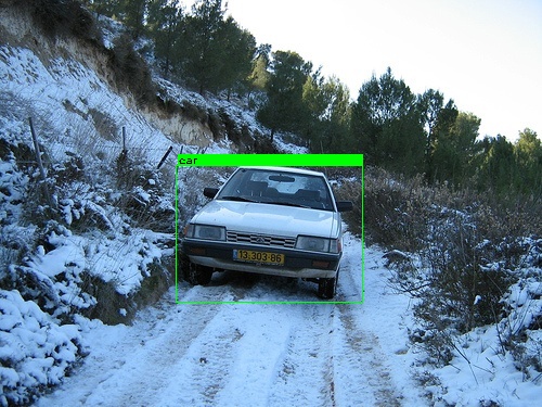
우선 훈련에 사용한 이미지에서는 다음과 같이 훌륭하게 나타납니다.

그런데 테스트용 데이터셋에서는 다음과 같이 나옵니다.

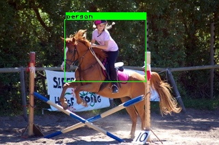
말을 탐지하지 못했군요. 이게 그나마 나은 결과고 아예 하나도 찾지 못하는 경우가 대다수였습니다. 제가 생각하기에는 nms에서 다 걸러진게 아닌가 싶습니다. 다른 방법을 사용해야하나 싶군요.

이런 현상이 발생한 이유는 너무 훈련용 데이터셋에 과적합 되었기 때문이 아닌가 싶습니다. 제가 훈련용 데이터셋에 데이터 증강을 적용하지 않았는데 데이터 증강을 적용했으면 테스트 데이터셋에서 더 좋은 결과를 얻지 않았을까 싶습니다.

구현 후기

---

생각보다 간단하면서도 삽질을 많이 했습니다. 특히 훈련을 시킬 때 엄청 삽질했습니다. 훈련 도중 loss가 무한대로 올라 NaN이 되어버려 모든 가중치도 NaN으로 조정되는 현상이 발생하는게 엄청 자주 일어나 꽤 힘들었습니다.

여러가지 방법을 쓰다가 결국 택한 방법이 NaN이 되기 전까지 훈련시키며 가중치를 저장하다가 NaN이 발생하면 훈련시키던 가중치를 불러온 뒤 이어서 훈련시키는 방법이었습니다. checkpoint가 가중치를 저장시키는 역할을 했죠.

그래도 뭔가 제대로 돌아가는 객체 탐지 모델을 만든건 이번이 처음입니다. 뿌듯합니다.
열심히 실력을 발전시켜 다음에는 더 정교하고 성능 좋은 모델을 만들 계획입니다.

지금까지 [YOLO 리뷰 + 구현]이었습니다.