• Three-dimensional plots are enabled by importing int mplot3d toolkit, included with the main Matplotlib installation.

# In[1]
from mpl_toolkits import mplot3d

• Once this submodule is imported, a three-dimensional axes can be created by passing the keyword projection='3d' to any of the normal axes creation routines.

# In[2]
%matplotlib inline
import numpy as np
import matplotlib.pyplot as plt

---

# In[3]
fig=plt.figure()
ax=plt.axes(projection='3d')

• With this three-dimensional axes enabled, we can now plot a variety of three-dimensional plot types.
• Three-dimensional plotting is one of the functionalities that benefits immensely from viewing figures interactively rather than statically, in the notebook; recall that to use interactive figures, you can use %matplotlib notebook rather than %matplotlib inline when running this code.

Three-Dimensional Points and Lines

• The most basic three-dimensional plot is a line or collection of scatter plots created from set of $(x,y,z)$ triples.
• In analogy with the more common two-dimensional plots, these can be created using the ax.plot3D and ax.scatter3D functions.

# In[4]
ax=plt.axes(projection='3d')

# data for a three-dimensional line
zline=np.linspace(0,15,1000)
xline=np.sin(zline)
yline=np.cos(zline)
ax.plot3D(xline, yline, zline, 'gray')

# data for three-dimensional scattered points
zdata=15 * np.random.random(100)
xdata=np.sin(zdata) + 0.1 * np.random.randn(100)
ydata=np.cos(zdata) + 0.1 * np.random.randn(100)
ax.scatter3D(xdata,ydata,zdata,c=zdata,cmap='Greens');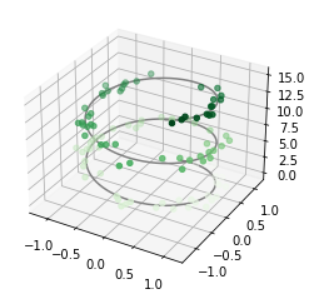

• Scatter points have their transparency adjusted to give a sense of depth on the page.
• While the three-dimensional effect is sometimes difficult to see within a static image, an interactive view can lead to some nice intuition about the layout of the points.

Three-Dimensional Contour Plots

• Analogous to the contour plots we explored in the last chapter, mplot3d contains tools to create three-dimensinal relief plots using the same inputs.
• Like ax.contour, ax.contour3D requires all the input data to be in the form of two-dimensional regular grids, with the $z$ data evaluated at each point.

# In[5]
def f(x,y):
    return np.sin(np.sqrt(x ** 2 + y ** 2))

x=np.linspace(-6,6,30)
y=np.linspace(-6,6,30)

X,Y=np.meshgrid(x,y)
Z=f(X,Y)

---

# In[6]
fig=plt.figure()
ax=plt.axes(projection='3d')
ax.contour3D(X,Y,Z,40,cmap='binary')
ax.set_xlabel('x')
ax.set_ylabel('y')
ax.set_zlabel('z');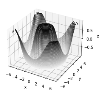

If you don't remember about np.meshgrid, refer to these urls :
1. numpy.meshgrid documentation
2. About meshgrid method

• Sometimes the default viewing angle is not optimal, in which case we can use the view_init method to set the elevation(높이) and azimuthal(방위각) angles.

# In[7]
ax.view_init(60,35)
fig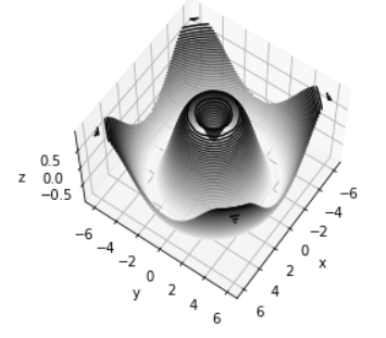

• We've use an elevation of 60 degrees (that is, 60 degrees above the x-y plane) and an azimuth of 35 degrees (that is, rotated 35 degrees counter-clockwise about the z-axis)
• This type of rotation can be accomplished interactively by clicking and dragging when using one of Matplotlib's interactive backends.

Wireframes and Surface Plots

• Two other types of three-dimensional plots that work on gridded data are wireframes and surface plots.
• These take a grid of values and project it onto the specified three-dimensional surface, and can make the resulting three-dimensional forms quite easy to visualize.

# In[8]
fig=plt.figure()
ax=plt.axes(projection='3d')
ax.plot_wireframe(X,Y,Z)
ax.set_title('wireframe');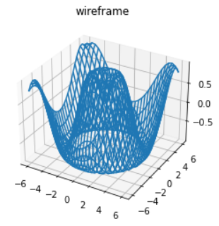

• A surface plot is like a wireframe plot, but each face of the wireframe is a filled polygon(다각형).
• Adding a colormap to the filled polygons can aid perception of the topology(체계적인 분류) of the surface being visualized.

# In[9]
ax=plt.axes(projection='3d')
ax.plot_surface(X,Y,Z,rstride=1,cstride=1,
cmap='viridis',edgecolor='none')
ax.set_title('surface');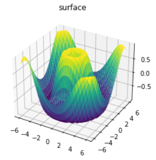

• Though the grid of values for a surface plot needs to be two-dimensional, it need not be rectilinear(직선으로 된).
• Creating a partial polar grid, which when used with the surface3D plot can give us a slice into the function we're visualizing.

# In[10]
r=np.linspace(0,6,20)
theta=np.linspace(-0.9 * np.pi, 0.8 * np.pi, 40)
r,theta=np.meshgrid(r,theta)

X = r * np.sin(theta)
Y = r * np.cos(theta)
Z = f(X,Y)

ax=plt.axes(projection='3d')
ax.plot_surface(X,Y,Z,rstride=1,cstride=1,
cmap='viridis',edgecolor='none');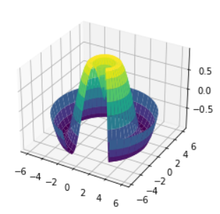

Surface Triangulations

• For some applications, the evenly sampled grids required by the preceding routines are too restrictive.
• In these situations, triangulation-based plots can come in handy.

# In[11]
theta = 2 * np.pi * np.random.random(1000)
r = 6 * np.random.random(1000)
x = np.ravel(r * np.sin(theta))
y = np.ravel(r * np.cos(theta))
z = f(x,y)

---

# In[12]
ax=plt.axes(projection='3d')
ax.scatter(x,y,z,c=z,cmap='viridis',linewidth=0.5);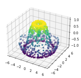

If you want to know about the np.ravel, refer to these urls :
1. numpy.ravel documentation
2. About ravel() and flatten()

• This point cloud leaves a lot to be desired.
• The function that will help us in this case is ax.plot_trisurf, which creates a surface by first finding a set of triangles formed between adjacent points.

# In[13]
ax=plt.axes(projection='3d')
ax.plot_trisurf(x,y,z,cmap='viridis',edgecolor='none');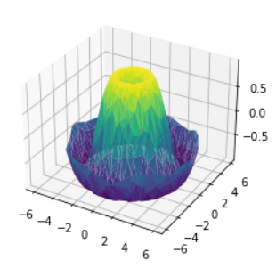

• The result is certainly not as clean as when it is plotted with a grid, but the flexibility of such triangulation allows for some really interesting three-dimensional plots.

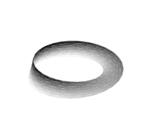
Example: Visualizing a Möbius strip

• The key to creating the Möbius strip is to think about its parametrization: it's a two-dimensional strip, so we need two intrinsic dimensions.
• We'll call them $\theta$, which ranges from 0 to $2\pi$ around the loop, and w, which ranges from -1 to 1 across the width of the strip.

# In[14]
theta=np.linspace(0, 2 * np.pi, 30)
w=np.linspace(-0.25,0.25,8)
w,theta=np.meshgrid(w,theta)

• From this parametrization, we must determine the (x,y,z) positions of the embedded strip.
  
  
• We might realize that there are two rotations happening: one is the position of the loop about its center (what we've called $\theta$), while the other is the twisting of the strip about its axis (we'll call this $\phi$).
• For a Möbius strip, we must have the strip make half a twist during a full loop, or $\delta\phi = \delta\theta/2$

# In[15]
phi = 0.5 * theta

• Now we use our recollection of trigonometry to derive the three-dimensional embedding.
• We'll define r, the distance of each point from the center, and use this to find the embedded (x,y,z) coordinates.

# In[16]
# radius in x-y plane
r = 1 + w * np.cos(phi)

x = np.ravel(r * np.cos(theta))
y = np.ravel(r * np.sin(theta))
z = np.ravel(w * np.sin(phi))

• Finally to plot the object, we must make sure the triangulation is correct.
• The best way to do this is to define the triangulation within the underlying parametrization, and then let Matplotlib project this triangulation into the three-dimensional space of the Möbius strip.

# In[17]
# triangulate in the underlying parametrization
from matplotlib.tri import Triangulation
tri=Triangulation(np.ravel(w),np.ravel(theta))

ax=plt.axes(projection='3d')
ax.plot_trisurf(x,y,z,triangles=tri.triangles,
cmap='Greys',linewidths=0.2);

ax.set_xlim(-1,1); ax.set_ylim(-1,1); ax.set_zlim(-1,1)
ax.axis('off');