Linear Regression

$\hat{y}$ = $w_0$ + $w_1$$x_1$
$y$: 실제값
$\hat{y}$: 예측값
$\bar{y}$: 평균값
$w_1$: 가중치(기울기)
$w_0$: 편향(y절편)

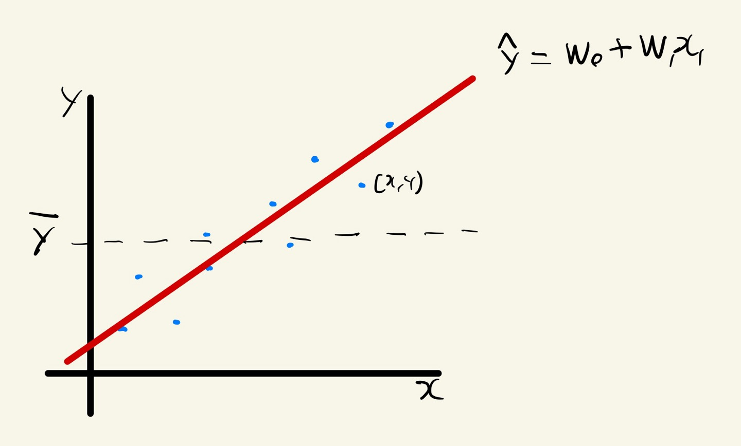
• 최적의 회귀모델은 전체 데이터의 오차 합의 최소가 되는 모델을 의미한다
• 독립변수 개수로 단순 회구와 다중 회귀로 분류

(1) 단순회귀

• 독립변수 하나가 종소변수에 영향을 미치는 선형 회귀
• 모델 학습 후 회귀계수 확인
• coef_ : 회귀계수(가중치)
• intercept_ : 편향
  y = -1 + 5.21x 로 표현

(2) 다중회귀

• 여러 독립변수가 종속변수에 영향을 미치는 선형 회귀
• 여러 개의 x값이 필요
  y = +9 + 2.65$x_1$ - 15.60$x_2$ + 1.16$x_3 으로 표현

(3) 모델구현

Linear Regression은 회귀모델에서만 사용 가능함

# 회귀모델 불러오기
from sklearn.linear_model import LinearRegression

# 회귀모델 평가지표 불러오기
from sklearn.metrics import mean_absolute_error, r2_score

K-Nearest Neighbor

• k 최근접 이웃

• 학습용 데이터에서 k개의 최근접 이웃을 찾아 그 값들로 새로운 값을 예측함

• k 값에 따라 예측 값이 달라져서 적절한 k 값 찾아야함

  • (n_neighbors=5)이 기본 값

• k를 1로 설정안함

• k를 홀수로 설정

• 회귀와 분류에 모두에 사용된다.

(1) 스케일링

• 스케일링 여부에 따라 KNN 모델 성능이 달라짐
• 평가용 데이터에도 학습용데이터를 기준으로 스케일링을 수행함

정규화 (Normalization)

• $\large x_{norm}=\frac{x-x_{min}}{x_{max}-x_{min}}$
• 각 변수의 값이 0과 1사이 값이 됨

# 정규화 전
plt.figure(figsize=(8, 2))
plt.boxplot(x_train, vert=False, labels=list(x))

plt.show()

# 정규화 방법 1
# 최댓값, 최솟값 구하기
x_max = x_train.max()
x_min = x_train.min()

# 정규화
x_train = (x_train - x_min) / (x_max - x_min) 
x_test = (x_test - x_min) / (x_max - x_min)


# 정규화 방법 2
# 모듈 불러오기
from sklearn.preprocessing import MinMaxScaler

# 정규화
scaler = MinMaxScaler()
# scaler.fit(x_train)
x_train = scaler.fit_transform(x_train)
x_test = scaler.transform(x_test)


# 정규화 후
plt.figure(figsize=(8, 2))
plt.boxplot(x_train, vert=False, labels=list(x))

plt.show()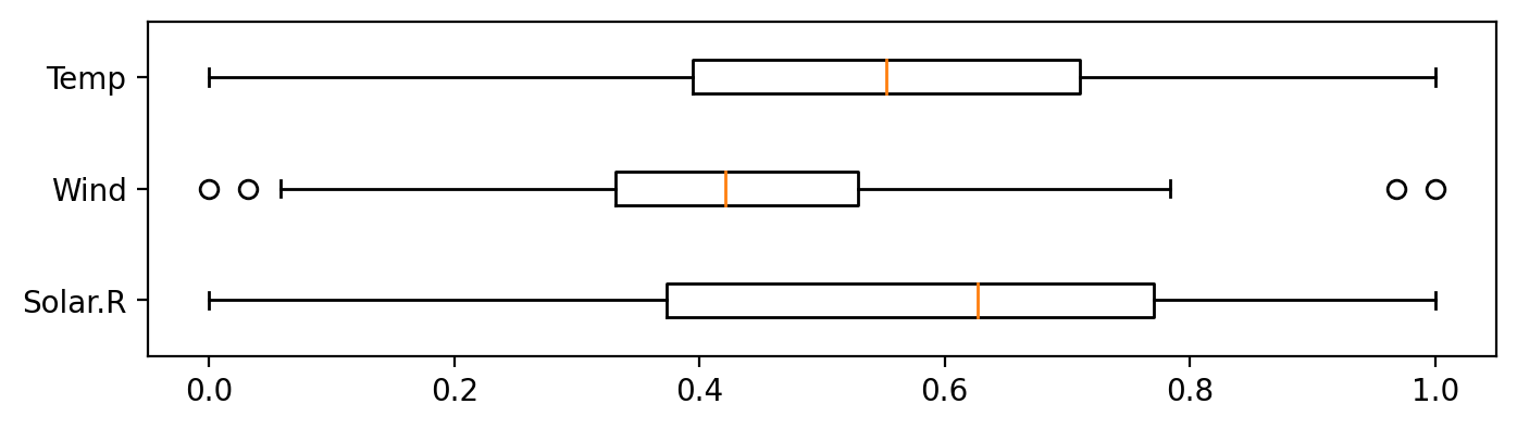

표준화 (Standardization)

• $\large x_{z}=\frac{x-x_{mean}}{x_{std}}$
• 각 변수의 평균이 0, 표준편차가 1이 됨

(2) 회귀 모델

• k개 값의 평균을 계산하여 값을 예측함

# 1단계: 불러오기
from sklearn.neighbors import KNeighborsRegressor
from sklearn.metrics import mean_absolute_error, r2_score

# 2단계: 선언하기
model = KNeighborsRegressor(n_neighbors=5)

# 3단계: 학습하기
model.fit(x_train, y_train)

# 4단계 예측하기
y_pred = model.predict(x_test)

# 5단계: 평가하기
print('Mae: ', mean_absolute_error(y_test, y_pred))
print('R2: ', r2_score(y_test, y_pred))

# 예측값, 실젯값 시각화
plt.plot(y_test.values, label='Actual')
plt.plot(y_pred, label='Predicted')
plt.legend()
plt.ylabel('Ozone')
plt.show()

• 시각화 하여 모델성능을 비교할 수 있음

(3) 분류 모델

• 가장 많이 포함된 유형으로 분류

# 1단계: 불러오기
from sklearn.neighbors import KNeighborsClassifier
from sklearn.metrics import confusion_matrix, classification_report

# 2단계: 선언하기
model = KNeighborsClassifier()

# 3단계: 학습하기
model.fit(x_train, y_train)

# 4단계: 예측하기
y_pred = model.predict(x_test)

# 5단계: 평가하기
print(confusion_matrix(y_test, y_pred))
print(classification_report(y_test, y_pred))

분류의 경우 시각화가 어려움

가변수화 (주의)

데이터프레임에서 x와 y 데이터를 분리하고 난 뒤
가변수화를 진행한다.

# 가변수화 대상: Gender, JobSatisfaction, MaritalStatus, OverTime
dum = ['Gender', 'JobSatisfaction', 'MaritalStatus', 'OverTime']

# 가변수화
x = pd.get_dummies(x, columns=dum, drop_first=True, dtype=int)

# 확인
x.head()

• 위 처럼 가변수화하는 데이터를 data가 아닌 x에 저장해줘야 한다.
• 이유는 이미 data라는 데이터프레임을 이미 x, y 분리하여 x에 저장했기 때문

Decision Tree

• 나무가지가 뻗는 형태로 분류해 나감
• 분류와 회귀 모두에 사용되는 지도학습 알고리즘
• 스케일링이나 전처리의 영향이 적음
• 과정을 눈으로 확인 가능(화이트박스모델)
• 과적합으로 모델 성능이 떨어지기 쉬움
• 트리깊이를 제한하는 가지치기 필요(max_depth)
• 분류 모델
  • 마지막 노드에 있는 샘플들의 최빈값을 예측값으로 반환
• 회귀 모델
  • MSE
  • 마지막 노드에 있는 샘플들의 평균을 예측값으로 반환

(1) 불순도

• 순도가 높을 수록 분류가 잘된 모델임
• 불순도 수치화 지표
  • 지니 불순도
    • 분류 후 얼마나 잘 분류했는지 평가하느 지표
    • 지니 불순도가 낮을수록 순도가 높음
    • 0 ~ 0.5 사이의 값
    • 완벽 분류의 경우 0
    • 완벽하게 섞이면 0.5
  • 엔트로피
    • 0 ~ 1 사이의 값
    • 완벽 분류의 경우 0
    • 완벽하게 섞이면 1

(2) 정보이득

• 정보이득이 크다 = 어떤 속성으로 분할할대 불순도가 줄어든다
• 정보이득이 가장 큰 속성부터 분할함

(3) 가지치기

• 색이 진할수록 분류가 잘된 것임
• max_depth, min_samples_leaf, min_samples_split
• 학습데이터 성능은 낮아지나, 평가데이터 성능 향상
• max_depth
  • 트리의 최대 깊이 (디폴트값 None)
• min_samples_split
  • 노드를 분할하기 위한 최소한의 샘플 개수 (디폴트값 2)
  • 과적합 방지 목적
• min_samples_leaf
  • 리프노드가 되기위한 최소한의 샘플 수 (디폴트값 1)

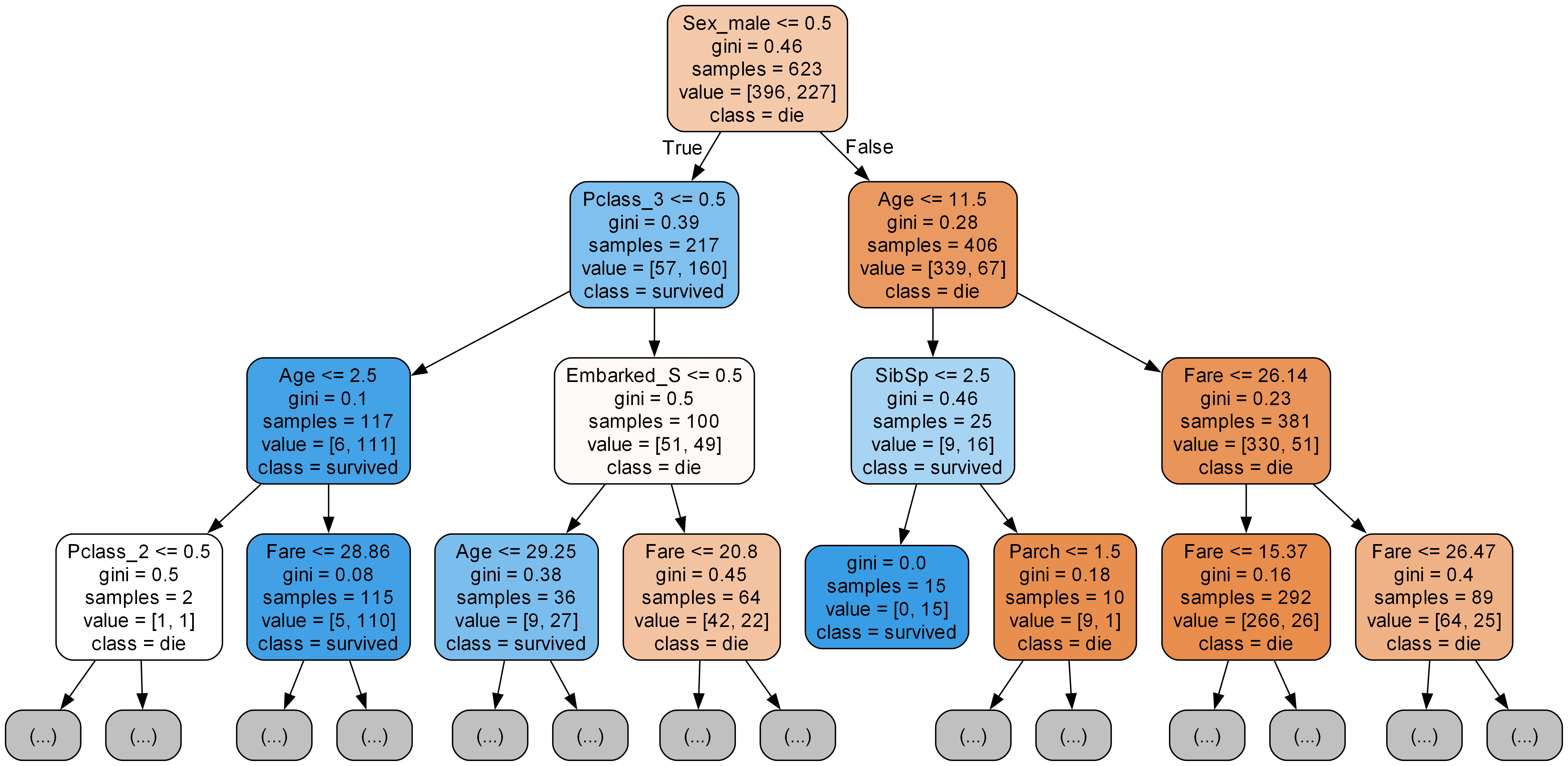
(4) 시각화 expot_graphviz

export_graphviz

# 시각화 모듈 불러오기
from sklearn.tree import export_graphviz
from IPython.display import Image

# 이미지 파일 만들기
export_graphviz(model,                                 # 모델 이름
                out_file='tree.dot',                   # 파일 이름
                feature_names=list(x),                 # Feature 이름
                class_names=['die', 'survived'],       # Target Class 이름
                rounded=True,                          # 둥근 테두리
                precision=2,                           # 불순도 소숫점 자리수
                max_depth=3,                           # 표시할 트리 깊이
                filled=True)                           # 박스 내부 채우기

# 파일 변환
!dot tree.dot -Tpng -otree.png -Gdpi=300

# 이미지 파일 표시
Image(filename='tree.png')

변수중요도 feature_importances_

• featureimportances 속성값으로 변수 중요도 확인
• 값이 클 수록 feature 의 중요도가 높음

# 변수 중요도
plt.figure(figsize=(5, 5))
plt.barh(list(x), model.feature_importances_)
# plt.barh(list(x), model.best_estimator_.feature_importances_)
plt.show()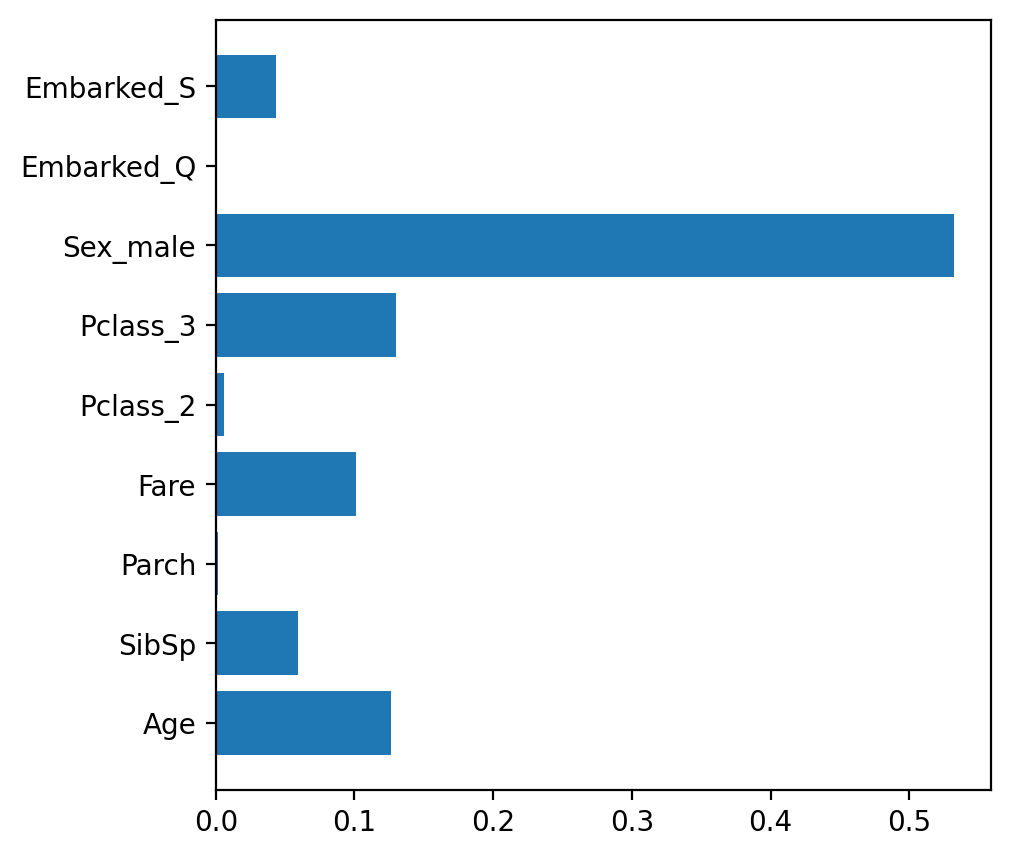

• 중요도를 기준으로 정렬

# 데이터프레임 만들기
df = pd.DataFrame()
df['feature'] = list(x)
df['importance'] = model.feature_importances_
df.sort_values(by='importance', ascending=True, inplace=True)

# 시각화
plt.figure(figsize=(5, 5))
plt.barh(df['feature'], df['importance'])
plt.show()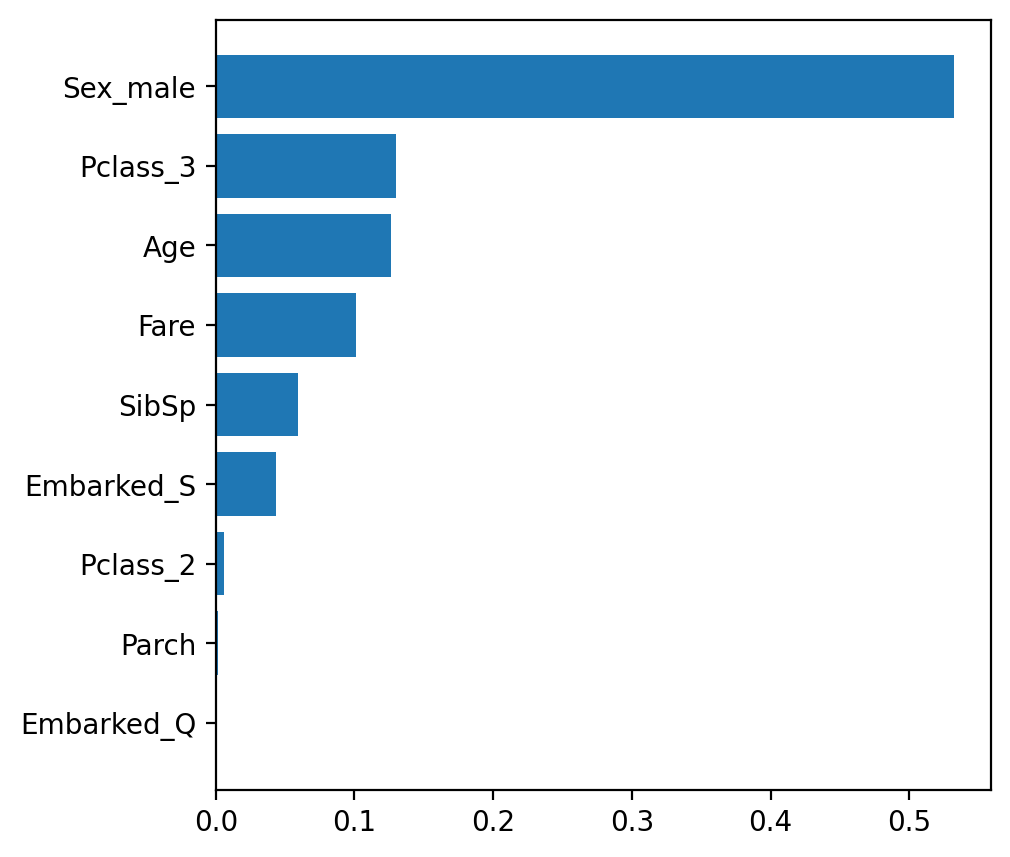

(5) 분류 모델 구현

# 1단계: 불러오기 
from sklearn.tree import DecisionTreeClassifier
from sklearn.metrics import confusion_matrix, classification_report

# 2단계: 선언하기
model = DecisionTreeClassifier(max_depth=5, random_state=1)

# 3단계: 학습하기
model.fit(x_train, y_train)

# 4단계: 예측하기
y_pred = model.predict(x_test)

# 5단계 평가하기
print(confusion_matrix(y_test, y_pred))
print(classification_report(y_test, y_pred))

(6) 회귀 모델 구현

# 1단계: 불러오기 
from sklearn.tree import DecisionTreeRegressor
from sklearn.metrics import mean_absolute_error, r2_score

# 2단계: 선언하기
model = DecisionTreeClassifier(max_depth=5)

# 3단계: 학습하기
model.fit(x_train, y_train)

# 4단계: 예측하기
y_pred = model.predict(x_test)

# 5단계 평가하기
print(mean_absolute_error(y_test, y_pred))
print(r2_score(y_test, y_pred))