미니프로젝트 1, 2일차

차량 공유 업체의 차량 사용 전 후에 촬영하는 차량의 정상/ 파손 이미지 무작위 수집을하여 분류하는 모델을 만들었다.

1. 데이터 전처리
2. CNN 모델링
3. Transfer learning

세가지 과제를 중점으로 수행하였다.

1. 데이터 전처리

먼저 데이터를 zip 파일 형식으로 불러와 압축해제하여 구글드라이브와 연결하여 불러오는 형식으로 진행하였다.

# 데이터 압축해제 함수
def dataset_extract(file_name) :
    with zipfile.ZipFile(file_name, 'r') as zip_ref :
        file_list = zip_ref.namelist()

        if os.path.exists(f'/content/{file_name[-14:-4]}/') :
            print(f'데이터셋 폴더가 이미 존재합니다.')
            return

        else :
            for f in tqdm(file_list, desc='Extracting', unit='files') :
                zip_ref.extract(member=f, path=f'/content/{file_name[-14:-4]}/')
                
# 구글 드라이브와 코랩 연결
from google.colab import drive
drive.mount('/content/drive')

# 데이터 압축해제 (경로 설정 중요)
dataset_extract('/content/drive/MyDrive/KT_deep_visualize/mini4/Car_Images.zip')

압축해제를 하면 Car_images가 구글 로컬환경에 생성되어 내부에 normal과 abnormal 폴더가 있다.

# 폴더별 이미지 데이터 갯수 확인
import glob

path = '/content/Car_Images/'

print(f'정상 차량 이미지 수: {len(glob.glob(path+"normal/*"))}' )
print(f'정상 차량 이미지 수: {len(glob.glob(path+"abnormal/*"))}' )

여기서 이미지 데이터는 glob.glob('경로')로 불러온다.

import random

# 정상 차량 랜덤 이미지 확인 및 형태 확인
rand_n = np.random.randint( 0, len(glob.glob(path+"normal/*"))-1 )

plt.figure(figsize=(5,5))
img = plt.imread(glob.glob(path+"normal/*")[rand_n])
plt.imshow(img)
plt.show()

print(f'이미지의 형태는 다음과 같다 : {img.shape}')


# 파손 차량 랜덤 이미지 확인 및 형태 확인
rand_n = np.random.randint( 0, len(glob.glob(path+"normal/*"))-1 )

plt.figure(figsize=(5,5))
img = plt.imread(glob.glob(path+"abnormal/*")[rand_n])
plt.imshow(img)
plt.show()

print(f'이미지의 형태는 다음과 같다 : {img.shape}')

이후 데이터 전처리를 위해 y변수에 정상차량은 0, 파손차량은 1로 하여 그 개수만큼 y_normal과 y_abnormal 변수에 0과 1을 넣어준다.

# 정상 차량은 0, 파손 차량은 1
y_normal = np.zeros((302,))
y_abnormal = np.ones((303,))

np.hstack() 을 사용하여 배열을 가로로 쌓아서 하나의 배열로 만들어준다.

# 정상 차량 어레이와 파손 차량 어레이 합치기
y_total = np.hstack((y_normal, y_abnormal))
y_total.shape

x 데이터 리스트를 통합한다.

x_total_list = glob.glob(path+"normal/*") + glob.glob(path+"abnormal/*")

x_total_list[:5]

데이터셋 분리

from sklearn.model_selection import train_test_split

# (1) train set, test set을 90:10의 비율로 분리
x_train, x_test, y_train, y_test =\
          train_test_split(x_total_list, y_total, test_size=0.1, random_state=2024)

x_train, x_val, y_train, y_val =\
          train_test_split(x_train, y_train, test_size=0.1, random_state=2024)

데이터를 모델링 하기 위해서는 np.array 형태로 데이터셋을 만들어야 한다.(reshape)
np.array로 만드는 함수를 생성해봄

import keras

# 데이터 reshape
def x_preprocessing(img_list) :
  bin_list = []

  for img in tqdm(img_list) :
    img = keras.utils.load_img( img, target_size=(128, 128) )
    img = keras.utils.img_to_array(img)
    bin_list.append(img)

  return np.array(bin_list)

x_tr_arr = x_preprocessing(x_train)
x_val_arr = x_preprocessing(x_val)
x_te_arr = x_preprocessing(x_test)

2. CNN 모델링

# 기본 CNN
# 1. 세션 클리어
clear_session()

# 2. 모델 선언
model1 = Sequential()

model1.add( Input(shape=(128, 128, 3)) )

model1.add( Conv2D(16, (3,3), (1,1), 'same', activation='relu') )
model1.add( BatchNormalization() )
model1.add( Dropout(0.4) )

model1.add( Conv2D(32, (3,3), (1,1), 'same', activation='relu') )
model1.add( MaxPool2D((2,2), (2,2)) )
model1.add( BatchNormalization() )
model1.add( Dropout(0.4) )

model1.add( Conv2D(64, (3,3), (1,1), 'same', activation='relu') )
model1.add( MaxPool2D((2,2), (2,2)) )
model1.add( BatchNormalization() )
model1.add( Dropout(0.4) )

model1.add( Flatten() )
model1.add( Dense(128, activation='relu') )
model1.add( Dense(1, activation='sigmoid'))

model1.compile(optimizer='adam',
               loss='binary_crossentropy',
               metrics=['accuracy']
               )
model1.summary()

이 방법으로 레이어층 마지막에 Dense를 더 겹겹이 쌓을수록 정확도가 높게 나왔다.

# Early Stopping

es = EarlyStopping(monitor='val_loss',
				   min_delta=0.3,
                   patience=10,
                   verbose=1,
                   restore_best_weights=True
                   )
model1.fit(x_tr_arr, y_train, validation_data=(x_val_arr, y_val),
		      epochs=10000,
          callbacks=[es]
          )
# 평가
model1.evaluate(x_te_arr, y_test)

# 예측
y_pred_1 = model1.predict(x_te_arr)
pred_1 = np.where(y_pred_1 >=0.5, 1, 0)

print(confusion_matrix(y_test, pred_1))
print(classification_report(y_test, pred_1))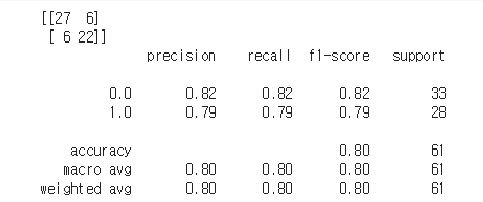

이런 결과가 나온다.

image_dataset_from_directory

from keras.utils import image_dataset_from_directory

idfd_train, idfd_valid = image_dataset_from_directory('/content/Car_Images/',
                                                      label_mode='binary',
                                                      image_size=(128,128),
                                                      shuffle=True,
                                                      seed=2024,
                                                      validation_split=0.2,
                                                      subset='both'
                                                      )

이걸 사용하여 Transfer learning을 진행할 것이다.

3. Transfer Learning

Inception V3

from keras.applications.inception_v3 import InceptionV3

base_model = InceptionV3(include_top=False,
                         weights='imagenet',
                         input_shape=(128,128,3)
                         )
base_model.trainable = False

base_model.layers[2].trainable = False

# 모델 구조 설계
## Functional API
clear_session()

i_l = Input(shape=(128,128,3))
aug = keras.layers.Rescaling(1./255)(i_l)
aug = keras.layers.RandomFlip()(aug)
aug = keras.layers.RandomRotation(0.2)(aug)

base = base_model(aug)

h_l = keras.layers.GlobalAvgPool2D()(base)
o_l = Dense(1, activation='sigmoid')(h_l)

model2 = Model(i_l, o_l)
model2.summary()

# 컴파일
model2.compile(optimizer='adam', loss='binary_crossentropy',
               metrics=['accuracy'])
               
# 학습
hist2 = model2.fit(idfd_train, validation_data=idfd_valid,
                   epochs=1000, verbose=1,
                   callbacks=[es, rlrp]
                   )

y_pred2 = model2.predict(x_te_arr)
y_pred2 = np.where(y_pred2>=0.5, 1, 0)

# 성능 평가
print( classification_report(y_test, y_pred2) )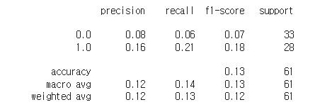

이미지 데이터수가 많이 작은 관계로 좋은 성능을 기대하기 어렵다.