https://github.com/nalinzip/ml_study/blob/main/ML_lastweek.ipynb

1. 추천 시스템의 개요와 배경

• 추천 엔진의 고도화는 수익 증대와 직결됨
• 전자상거래 업체는 추천 시스템 도입으로 매출 증가 경험
• 추천 시스템은 사용자 쇼핑의 즐거움도 증대시킴
• 유튜브, 애플 뮤직은 클릭 몇 번으로 연관 콘텐츠를 연속 추천
• 잊고 있던 취향이나 새로운 취향의 콘텐츠도 발견 가능
• 고도화된 추천 엔진은 사이트에서 쉽게 빠져나올 수 없게 만듦
• 추천 콘텐츠는 개인적 취향을 잘 반영함
• 추천 콘텐츠의 연관성과 맞춤성은 사이트 평판에 중요한 요소
• 추천 시스템의 묘미는 사용자가 인식하지 못한 취향까지 찾아주는 데 있음

온라인 스토어의 필수 요소, 추천 시스템

• 온라인에서 추천 시스템은 필수
• 상품이 너무 많아 사용자가 선택에 어려움
• 선택 부담은 쇼핑 피로와 매출 감소로 이어짐
• 추천 시스템이 빠르게 관심 상품을 제안
• 사용자 경험 향상 및 구매 유도
• 고객 데이터로 맞춤 추천 가능

예를 들어 다음과 같은 데이터가 추천 시스템을 구성하는 데 사용

• 사용자가 어떤 상품을 구매했는가?
• 사용자가 어떤 상품을 둘러보거나 장바구니에 넣었는가?
• 사용자가 평가한 영화 평점은? 제품 평가는?
• 사용자가 스스로 작성한 자신의 취향은?
• 사용자가 무엇을 클릭했는가?

이러한 데이터를 기반으로 추천 시스템은

• ‘당신만을 위한 최신 상품’,
• ‘이 상품을 선택한 다른 사람들이 좋아하는 상품들’,
• ‘이 상품을 좋아하나요? 아래 있는 다른 상품은 어떤가요?’
  와 같은 친숙한 문구로 사용자가 상품을 구매하도록 유혹함

2. 콘텐츠 기반 필터링 추천 시스 템

• 콘텐츠 기반 필터링은 사용자가 선호한 아이템과 유사한 콘텐츠를 가진 다른 아이템을 추천
• 예: ‘컨택트’(SF, 미스터리), ‘프로메테우스’(SF, 액션, 스릴러)에 높은 점수를 준 경우
• 추천 시스템은 장르, 감독, 출연진, 키워드 등을 분석
• 유사 콘텐츠를 가진 ‘블레이드 러너 2049’와 같은 영화를 추천 가능

3. 최근접 이웃 협업 필터링

• 신작 영화 선택은 시간·비용 부담이 크므로, 예고편·전문가 평·감독 등만 보고 결정 시 실망할 수 있음
• 따라서 취향이 비슷한 친구들의 평가를 참고하는 것이 일반적임
• 이처럼 사용자 행동(평점, 구매 이력 등)을 바탕으로 추천하는 방식이 협업 필터링임
• 협업 필터링은 사용자–아이템 평점 행렬을 기반으로, 평가하지 않은 아이템의 예측 평점을 계산
• 이 평점 행렬은 희소 행렬(Sparse Matrix) 구조를 가지며, 데이터가 부분적으로만 채워져 있음

최근접 이웃 협업 필터링은 메모리(Memory) 협업 필터링이라고도 하며,
일반적으로 사용자 기반과 아이템 기반으로 다시 나뉠 수 있음

• 사용자 기반 (User-User):
  “당신과 비슷한 고객들이 다음 상품도 구매했습니다.”
  (Customers like you also bought these items)

• 아이템 기반 (Item-Item):
  “이 상품을 선택한 다른 고객들은 다음 상품도 구매했습니다.”
  (Customers who bought this item also bought these items)

• 사용자 기반 최근접 이웃 방식은 특정 사용자와 유사한 다른 사용자를 TOP-N으로 선정해,
  이 Top-N 사용자가 좋아하는 아이템을 추천하는 방식임

• 즉, 특정 사용자와 타 사용자 간의 유사도(Similarity)를 측정한 뒤,
  가장 유사도가 높은 Top-N 사용자를 추출해 그들이 선호하는 아이템을 추천함

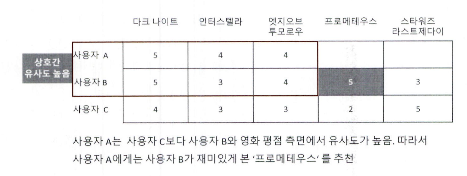
• 다음 그림은 사용자별 영화 평점 정보를 나타내고 있음
  

• 사용자 A는 주요 영화의 평점 정보가 사용자 C보다 사용자 B와 비슷하므로, 사용자 A와 사용자 B는 상호 간 유사도가 매우 높다고 할 수 있음

• 만약 사용자 A에게 아직 보지 못한 두 개의 영화인 ‘프로메테우스’와 ‘스타워즈 – 라스트 제다이’ 중 하나를 추천한다면, 사용자 C가 재미있게 본 ‘스타워즈 – 라스트 제다이’보다는, 사용자 A와 유사도가 높은 사용자 B가 재미있게 관람한 ‘프로메테우스’를 추천하는 것이 사용자 기반 최근접 이웃 협업 필터링임

• 아이템 기반 최근접 이웃 방식은 그 명칭이 주는 이미지 때문에 ‘아이템 간의 속성이 얼마나 비슷한지를 기반으로 추천한다’고 착각할 수 있음

• 하지만 아이템 기반 최근접 이웃 방식은 아이템이 가지는 속성과는 상관없이,
  사용자들이 그 아이템을 좋아하는지 / 싫어하는지의 평가 척도가 유사한 아이템을 추천하는 기준이 되는 알고리즘임

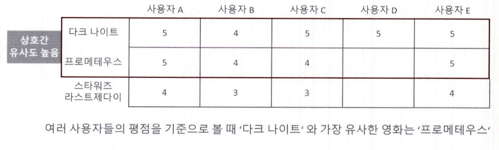
아이템 기반 최근접 이웃 방식의 기반 데이터셋입니다.

위의 사용자 기반 최근접 이웃 데이터셋과 행과 열이 서로 반대입니다.
(행이 개별 아이템이고, 열이 개별 사용자)

• 아이템(영화) ‘다크 나이트’는 ‘스타워즈 – 라스트 제다이’보다 ‘프로메테우스’와 사용자들의 평점 분포가 훨씬더 비슷하므로, ‘다크 나이트’와 ‘프로메테우스’는 상호 간 아이템 유사도가 상대적으로 매우 높음

• 따라서 ‘다크 나이트’를 매우 좋아하는 사용자 D에게, 아이템 기반 협업 필터링은 D가 아직 관람하지 못한 ‘프로메테우스’와 ‘스타워즈 – 라스트 제다이’ 중 ‘프로메테우스’를 추천함

• 일반적으로 사용자 기반보다는 아이템 기반 협업 필터링이 정확도가 더 높음

• 이유는 비슷한 영화를 좋아하거나 상품을 구입했다고 해서 사람들의 취향이 반드시 비슷하다고 판단하기 어려운 경우가 많기 때문임

• 매우 유명한 영화는 취향과 관계없이 대부분의 사람이 관람하는 경우가 많고, 사용자들이 평점을 매긴 영화(또는 상품)의 개수가 많지 않은 경우가 일반적이며, 이를 기반으로 다른 사람과의 유사도를 비교하기가 어려운 부분도 있음

• 따라서 최근접 이웃 협업 필터링은 대부분 아이템 기반 알고리즘을 적용함

4. 잠재 요인 협업 필터링

• 잠재 요인 협업 필터링은 사용자–아이템 평점 행렬에서 잠재 요인을 추출해 추천을 예측하는 기법임
• 대규모 행렬을 SVD 등 차원 축소 기법으로 분해하여 잠재 요인을 도출함
• 이러한 방식은 행렬 분해(Matrix Factorization) 라고 불림
• 넷플릭스 경연대회 우승 모델에 적용되어 유명해졌으며, 이후 널리 활용됨
• 잠재 요인은 평점 데이터만으로 도출되며, 구체적으로 정의되기보다는 수학적으로 계산되는 특성임

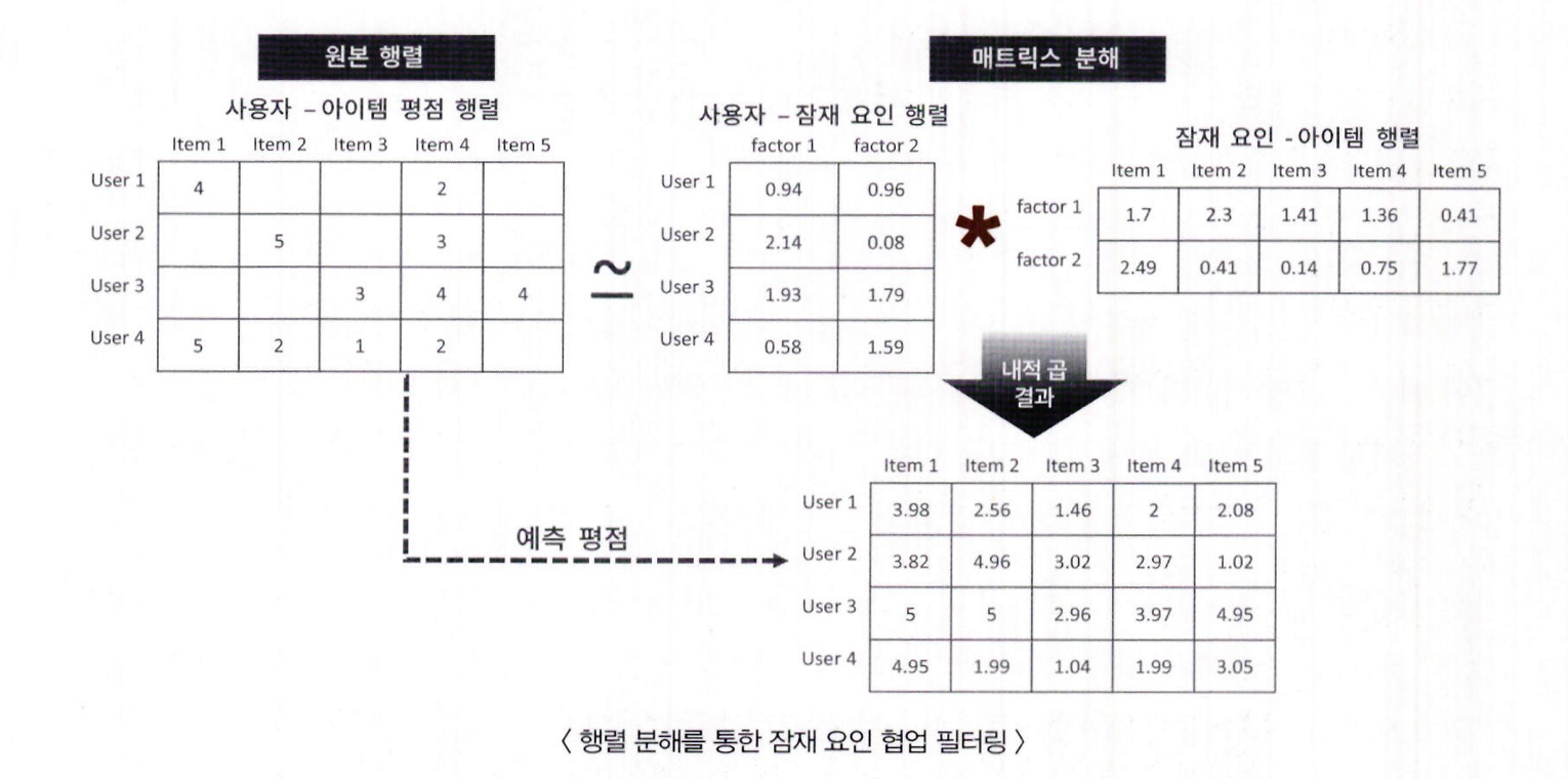
• 잠재 요인 협업 필터링은 사용자–아이템 희소 행렬을 저차원 밀집 행렬 두 개로 분해함
• 하나는 사용자–잠재 요인 행렬, 다른 하나는 아이템–잠재 요인 행렬의 전치 행렬(잠재 요인–아이템 행렬)임
• 이 두 행렬의 내적(dot product)을 통해 새로운 예측 사용자–아이템 평점 행렬을 생성함
• 이를 통해 사용자가 아직 평가하지 않은 아이템의 예측 평점을 계산할 수 있음
• 이 방식은 잠재 요인 기반 협업 필터링 알고리즘의 핵심 원리임

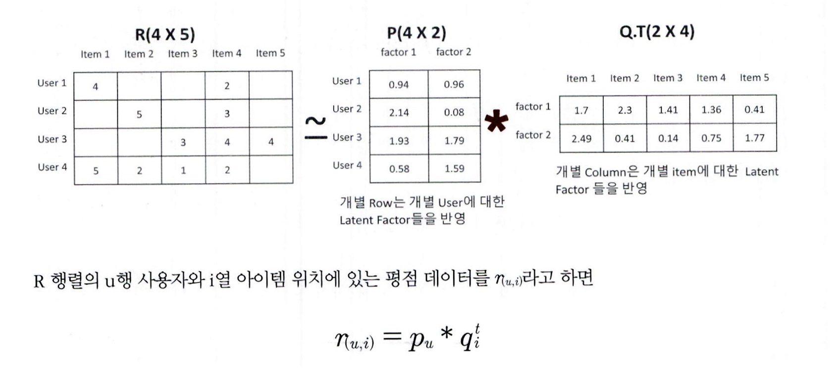
• 행렬 분해로 추출되는 '잠재 요인'은 명확히 정의할 수는 없지만, 예를 들어 영화의 경우 장르별 특성 선호도로 가정 가능함
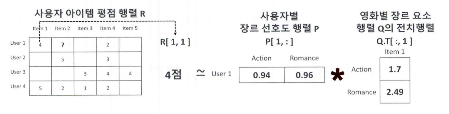
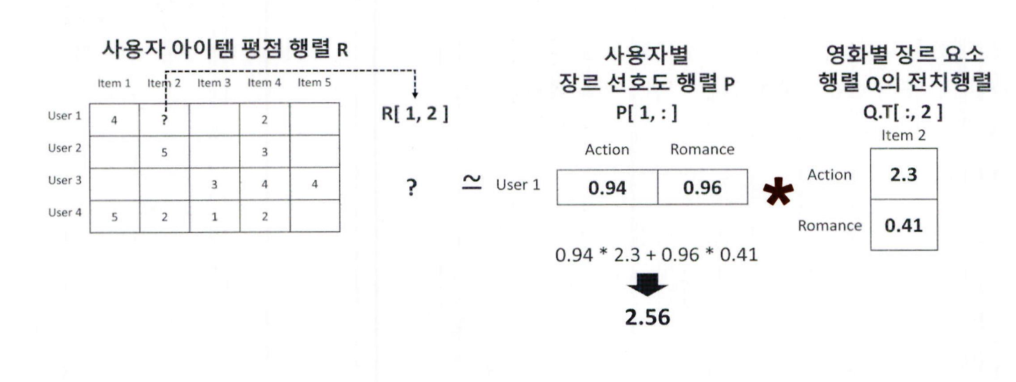
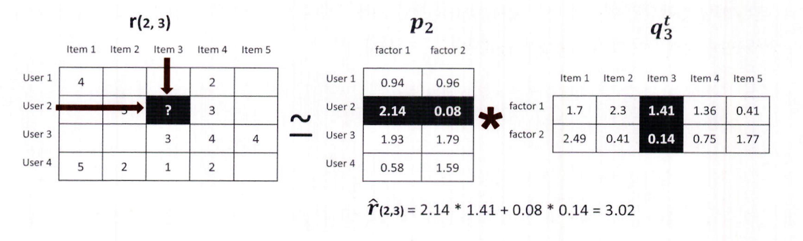
• 사용자–아이템 평점 행렬 R(u, i)에서 u는 사용자, i는 아이템이며, 예: R(1, 1) = 4, R(1, 4) = 2
• 사용자–잠재 요인 행렬 P(u, k)는 사용자의 장르별 선호도를 의미함

예: factor1 = 액션 선호도, factor2 = 로맨스 선호도

예: P(1, 1) = 0.94 (사용자 1의 액션 선호도), P(1, 2) = 0.96 (로맨스 선호도)

• 아이템–잠재 요인 행렬 Q(i, k)는 영화의 장르별 구성 요소 값을 의미함
• factor1 = 액션 요소, factor2 = 로맨스 요소
• 행렬 내적을 위해 전치(Q.T)하여 사용함

예: Q.T(1, 1) = 1.7 (영화 1의 액션 요소), Q.T(2, 1) = 2.49 (영화 2의 액션 요소)

• 평점은 사용자의 특정 장르 선호도와 영화의 그 장르적 특성을 반영하여 결정됨
  예: 사용자가 액션 장르를 매우 좋아하고, 영화가 액션 특성이 크면 높은 평점을 줄 가능성이 높음

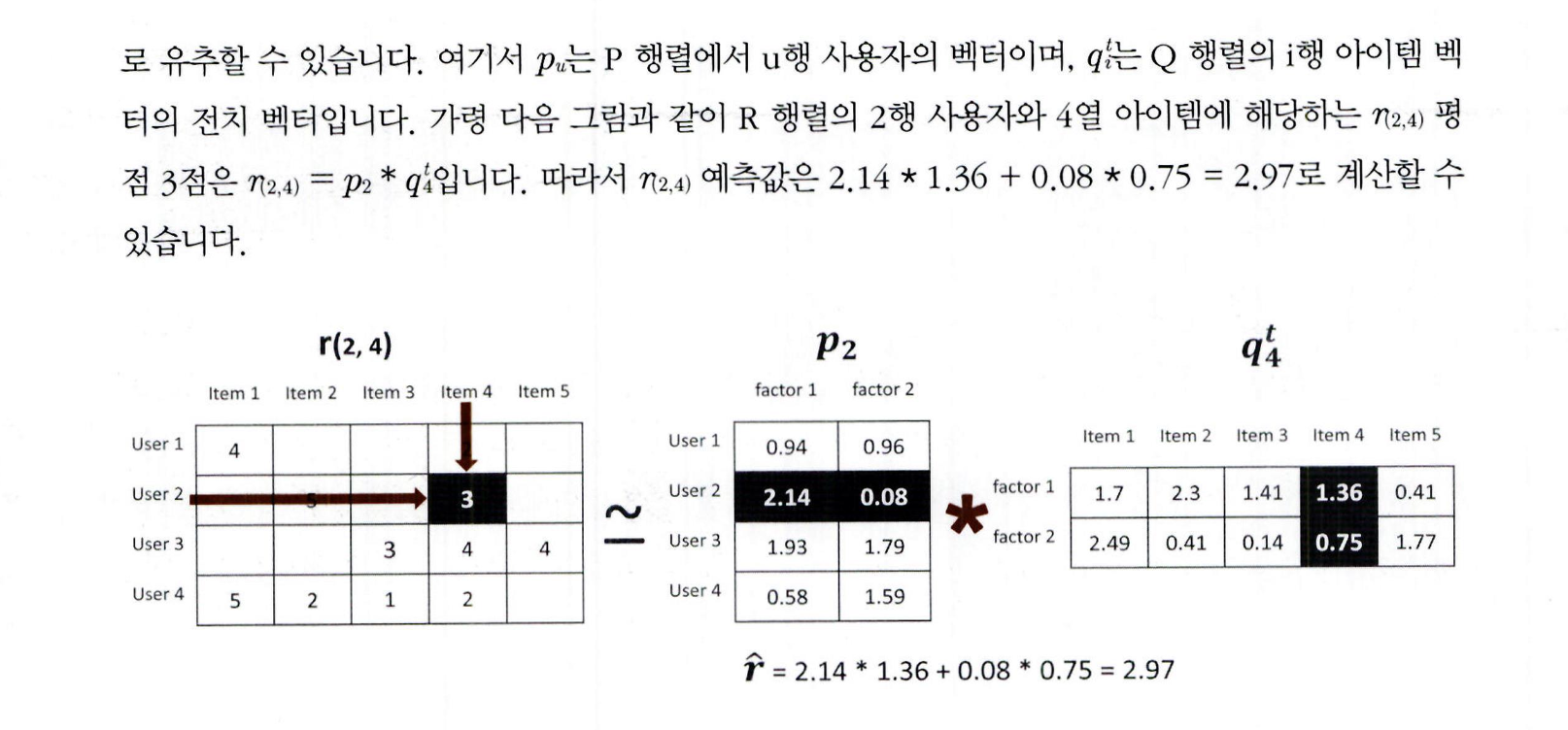
• 평점은 사용자 선호도 벡터(P)와 영화 특성 벡터(Q.T)의 내적 결과로 계산 가능

예: R(1, 1) = 4는 P 매트릭스의 User 1 벡터와 Q.T 매트릭스의 Item 1 벡터의 내적 결과

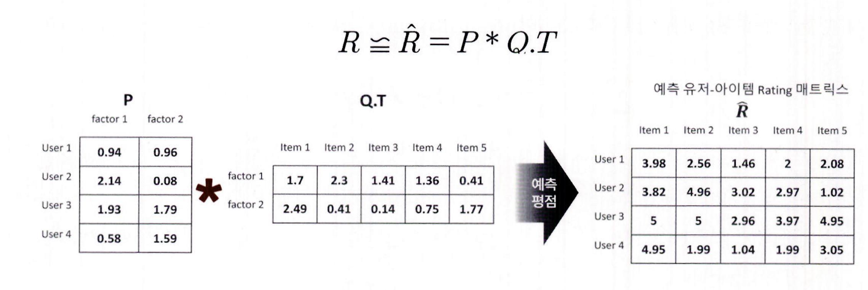
• 아직 평점을 매기지 않은 Item 2에 대해서도 같은 방식으로 예측 가능

예: R(1, 2) = 2.56 (User 1의 벡터와 Item 2 벡터의 내적 결과)

• 잠재 요인 협업 필터링은 숨겨진 잠재 요인을 기반으로
• 분해된 매트릭스를 이용해 사용자가 평가하지 않은 아이템의 예측 평점을 수행함
• 사용자–아이템 평점 행렬처럼 다차원 매트릭스를
• 저차원 매트릭스로 분해하는 기법을 행렬 분해(Matrix Factorization)라고 함

행렬 분해의 이해

• 행렬 분해(Matrix Factorization)는 다차원 행렬을 저차원 행렬로 분해하는 기법임
• 대표적인 방법으로는 SVD(Singular Value Decomposition), NMF(Non-Negative Matrix Factorization) 등이 있음
• 인수 분해란 복잡한 다항식을 단순한 인수의 곱으로 표현하는 것으로, 예: x² + 5x + 6 → (x + 2)(x + 3)
• 행렬 분해도 이와 유사하며, 대상만 행렬일 뿐
• 사용자–아이템 평점 행렬 R (M×N 차원)은 사용자–잠재 요인 행렬 P (M×K 차원)와 잠재 요인–아이템 행렬 Q.T (K×N 차원)로 분해됨

여기서 Q는 아이템–잠재 요인 행렬 (N×K 차원), Q.T는 그 전치 행렬임

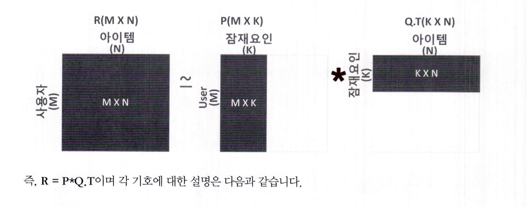
M: 총 사용자 수

N: 총 아이템 수

K: 잠재 요인의 차원 수

R (M×N): 사용자–아이템 평점 행렬

P (M×K): 사용자와 잠재 요인 간 관계 값을 담은 행렬

Q (N×K): 아이템과 잠재 요인 간 관계 값을 담은 행렬

Q.T (K×N): Q 행렬의 전치 행렬

예시: 많은 널(NaN) 값을 가지는 고차원의 희소 행렬 R은
→ 저차원의 밀집 행렬 P와 Q로 분해될 수 있음

사용자-아이템 평점 행렬의 미정 값을 포함한 모든 평점 값은 행렬 분해를 통해 얻어진 P 행렬과 Q.T 행렬의 내적을 통해 예측 평점으로 다시 계산할 수 있음

• R 행렬을 P와 Q 행렬로 분해하려면 SVD(Singular Value Decomposition) 방식이 일반적으로 사용됨
• 하지만 SVD는 널(NaN) 값이 없는 행렬에만 적용 가능
• R 행렬에는 평가되지 않은 항목이 많아 일반적인 SVD는 적용 불가
• 이 경우, SGD(Stochastic Gradient Descent) 또는 ALS(Alternating Least Squares) 방식으로 행렬 분해 수행

확률적 경사하강법을 이용한 행렬 분해

• 확률적 경사 하강법(SGD)은 경사 하강법의 일종으로, 5장 회귀의 3절에서 소개된 개념임

• SGD를 활용한 행렬 분해는 예측 행렬(R̂)이 실제 행렬(R)과 최소한의 오류를 갖도록 비용 함수 최적화를 반복

• 절차:

P와 Q 행렬을 임의의 값으로 초기화
P와 Q.T의 곱으로 예측 R 행렬을 계산하고 오류 측정
이 오류를 최소화하기 위해 P와 Q 값을 반복적으로 업데이트
오류가 충분히 줄어들 때까지 2, 3단계를 반복

• 최적화 시 L2 규제를 포함한 비용 함수도 고려됨

• 5장 3절의 회귀 경사 하강법에서는 비용 함수 최소화를 위해 계수 업데이트(w₁_update, w₀_update)를 반복적으로 적용함
• 행렬 분해도 유사하게, SGD 기반으로 예측 R과 실제 R의 차이(오차)를 최소화하는 방향으로 P, Q 행렬을 반복 갱신함
• 핵심: L2 규제를 포함한 비용 함수 최소화
• 목표: 최적화된 예측 행렬 R̂ = P × Qᵀ
• 구현 계획:

원본 행렬 R을 np.NaN 포함하여 생성
분해할 행렬 P, Q는 정규 분포 기반 랜덤 값으로 초기화
잠재 요인 차원 수 K는 3으로 설정
이후 반복 최적화를 통해 P와 Q를 학습하고, P @ Q.T로 예측 행렬 생성

import numpy as np

# 원본 행렬 R 생성, 분해 행렬 P와 Q 초기화, 잠재요인 차원 K는 3 설정.
R = np.array([[4, np.nan, np.nan, 2, np.nan ],
              [np.nan, 5, np.nan, 3, 1 ],
              [np.nan, np.nan, 3, 4, 4 ],
              [5, 2, 1, 2, np.nan ]])
num_users, num_items = R.shape
K=3

# P와 Q 매트릭스의 크기를 지정하고 정규분포를 가진 random한 값으로 입력합니다.
np.random.seed(1)
P = np.random.normal(scale=1./K, size=(num_users, K))
Q = np.random.normal(scale=1./K, size=(num_items, K))
     

다음으로 실제 R 행렬과 예측 행렬의 오차를 구하는 get_rmse() 함수를 만들어보겠습니다.

• get_rmse() 함수는 실제 R 행렬의 널이 아닌 행렬 값의 위치 인덱스를 추출
• 이 인덱스에 있는 실제 R 행렬 값과 분해된 P, Q를 이용해 다시 조합된 예측 행렬 값의 RMSE 값을 반환

from sklearn.metrics import mean_squared_error

def get_rmse(R, P, Q, non_zeros):
    error = 0
    # 두개의 분해된 행렬 P와 Q.T의 내적으로 예측 R 행렬 생성
    full_pred_matrix = np.dot(P, Q.T)

    # 실제 R 행렬에서 널이 아닌 값의 위치 인덱스 추출하여 실제 R 행렬과 예측 행렬의 RMSE 추출
    x_non_zero_ind = [non_zero[0] for non_zero in non_zeros]
    y_non_zero_ind = [non_zero[1] for non_zero in non_zeros]
    R_non_zeros = R[x_non_zero_ind, y_non_zero_ind]
    full_pred_matrix_non_zeros = full_pred_matrix[x_non_zero_ind, y_non_zero_ind]

    mse = mean_squared_error(R_non_zeros, full_pred_matrix_non_zeros)
    rmse = np.sqrt(mse)

    return rmse

SGD 기반 행렬 분해 과정 요약:

• R 행렬에서 NaN이 아닌 실제 평점이 존재하는 (user, item) 인덱스를 추출
• 주요 하이퍼파라미터 설정:
  steps = 1000 (반복 횟수)
  learning_rate = η (학습률)
  r_lambda = λ (L2 규제 계수)

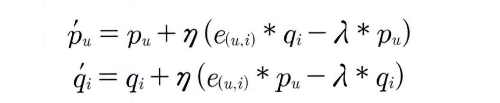
업데이트 식:

사용자 벡터 pu 업데이트:
pu = pu + η (e_ui qi - λ * pu)

아이템 벡터 qi 업데이트:
qi = qi + η (e_ui pu - λ * qi)

오류 출력:

get_rmse() 함수를 사용

50회마다 RMSE(평균 제곱근 오차)를 출력해 학습 성능 확인

# R > 0 인 행 위치, 열 위치, 값을 non_zeros 리스트에 저장.
non_zeros = [ (i, j, R[i,j]) for i in range(num_users) for j in range(num_items) if R[i,j] > 0 ]

steps=1000
learning_rate=0.01
r_lambda=0.01

# SGD 기법으로 P와 Q 매트릭스를 계속 업데이트.
for step in range(steps):
    for i, j, r in non_zeros:
        # 실제 값과 예측 값의 차이인 오류 값 구함
        eij = r - np.dot(P[i, :], Q[j, :].T)
        # Regularization을 반영한 SGD 업데이트 공식 적용
        P[i,:] = P[i,:] + learning_rate*(eij * Q[j, :] - r_lambda*P[i,:])
        Q[j,:] = Q[j,:] + learning_rate*(eij * P[i, :] - r_lambda*Q[j,:])

    rmse = get_rmse(R, P, Q, non_zeros)
    if (step % 50) == 0 :
        print("### iteration step : ", step," rmse : ", rmse)

이제 분해된 P와 Q 행렬을 P * Q.T로 곱하여 예측 행렬을 만들어서 출력

pred_matrix = np.dot(P, Q.T)
print('예측 행렬:\n', np.round(pred_matrix, 3))

SGD로 분해한 예측 행렬 결과:

• 원본 행렬의 널이 아닌 값들과 비교해 큰 차이가 없음
• 널 값들은 새로운 예측 값으로 채워짐

활용 예고:

• 7절에서는 이 예제 기반으로 사용자–영화 평점 행렬을 행렬 분해하고 영화 추천 로직 구현에 활용할 예정임

5. 콘텐츠 기반 필터링 실습 - TMDB5000 영 화 데이터세트

장르 속성을 이용한 영화 콘텐츠 기반 필터링

• 콘텐츠 기반 필터링은 사용자가 좋아한 영화와 유사한 특성을 가진 영화를 추천함
• 예: ‘인셉션’을 좋아했다면, 장르(액션, 공상과학) 또는 감독(크리스토퍼 놀란) 기반으로 유사한 영화 추천
• 영화 간 유사성 판단 기준은 장르, 감독, 배우, 평점, 키워드, 설명 등 콘텐츠 정보
• 추천 방식은 장르 칼럼의 유사도 비교 후, 높은 평점을 받은 영화 추천

import pandas as pd
import numpy as np
import warnings; warnings.filterwarnings('ignore')

movies =pd.read_csv('/content/sample_data/tmdb_5000_movies.csv')
print(movies.shape)
movies.head(1)

• tmdb_5000_movies.csv는 총 4,803개의 레코드와 20개의 피처로 구성됨
• 영화에 대한 메타 정보는 제목, 개요, 인기도, 평점, 투표 수, 예산, 키워드 등을 포함함
• 콘텐츠 기반 필터링 추천 분석을 위해 주요 칼럼만 추출해 DataFrame 생성

주요 칼럼:
id
title (영화 제목)
genres (영화 장르)
vote_average (평균 평점)
vote_count (평점 투표 수)
popularity (인기도)
keywords (주요 키워드 문구)
overview (영화 개요 설명)

movies_df = movies[['id','title', 'genres', 'vote_average', 'vote_count',
                 'popularity', 'keywords', 'overview']]
     

• tmdb_5000_movies.csv 파일에서 genres, keywords 칼럼은 다음과 같은 형태의 문자열로 저장됨:
  "[{"id": 28, "name": "Action"}, {"id": 12, "name": "Adventure"}]"
• 이는 파이썬의 리스트 안에 딕셔너리가 여러 개 들어 있는 구조지만, 실제로는 문자열로 읽혀짐
• 예: 영화 ‘아바타’의 genres는 ["Action", "Adventure", ...] 식의 복수 장르를 표현
• 하지만 DataFrame에 로딩되면 단순 문자열로 취급되므로, 이를 파싱하지 않으면 정보 추출 불가능
• 따라서 genres, keywords 등의 칼럼은 가공(parse) 작업이 필요
• 우선 해당 칼럼이 실제로 어떤 형태인지 직접 확인하는 작업이 선행되어야 함

pd.set_option('max_colwidth', 100)
movies_df[['genres','keywords']][:1]

• genres 칼럼은 각 영화가 속한 여러 장르 정보를 리스트 안의 딕셔너리 형태로 문자열로 저장하고 있음
  예: [{"id": 28, "name": "Action"}, {"id": 12, "name": "Adventure"}]
• keywords 칼럼도 동일한 구조를 가짐
• 이 문자열을 실제 파이썬 객체로 변환하려면 ast.literal_eval() 함수 사용
• pandas.Series.apply()와 함께 literal_eval()을 사용하면 DataFrame 내 각 셀의 문자열을 파이썬 리스트로 변환 가능
• 목적은 각 딕셔너리에서 'name' 값을 추출하여 리스트로 구성하는 것임
• 예:
  원본 문자열 → [{"id": 28, "name": "Action"}, {"id": 12, "name": "Adventure"}]
  변환 결과 → ['Action', 'Adventure']

from ast import literal_eval

movies_df['genres'] = movies_df['genres'].apply(literal_eval)
movies_df['keywords'] = movies_df['keywords'].apply(literal_eval)
     

• genres 칼럼은 리스트 내부에 여러 딕셔너리로 구성된 객체를 가짐
• 예: [{"id": 28, "name": "Action"}, {"id": 12, "name": "Adventure"}]
• 이를 ['Action', 'Adventure'] 형태로 변환해야 함
• 방법:
  apply()와 lambda 함수 사용
  코드 예시: apply(lambda x: [y['name'] for y in x])
  리스트 내 딕셔너리에서 'name' 키 값만 추출하여 리스트로 변환함

movies_df['genres'] = movies_df['genres'].apply(lambda x : [ y['name'] for y in x])
movies_df['keywords'] = movies_df['keywords'].apply(lambda x : [ y['name'] for y in x])
movies_df[['genres', 'keywords']][:1]
     

• genres 칼럼은 여러 개의 개별 장르가 리스트로 구성돼 있음
• 영화 A의 genres: [Action, Adventure, Fantasy, Science Fiction]
• 영화 B의 genres: [Adventure, Fantasy, Action]
• 장르별 유사도 측정 방법: genres를 문자열로 변경한 뒤 CountVectorizer로 피처 벡터화한 행렬 데이터를 코사인 유사도로 비교

콘텐츠 기반 필터링 구현 단계:

• 문자열로 변환된 genres 칼럼을 Count 기반으로 피처 벡터화 변환

• genres 문자열을 피처 벡터화 행렬로 변환한 데이터셋을 코사인 유사도를 통해 비교

• 장르 유사도가 높은 영화 중에 평점이 높은 순으로 영화를 추천

• 리스트 객체 값으로 구성된 genres 칼럼에 apply(lambda x: (' ').join(x))를 적용해 개별 요소를 공백 문자로 구분하는 문자열로 변환해 별도의 칼럼인 genres_literal 칼럼으로 저장

• 리스트 객체 내의 개별 값을 연속된 문자열로 변환하려면 일반적으로 ('구분문자').join(리스트 객체)를 사용

from sklearn.feature_extraction.text import CountVectorizer

# CountVectorizer를 적용하기 위해 공백문자로 word 단위가 구분되는 문자열로 변환.
movies_df['genres_literal'] = movies_df['genres'].apply(lambda x : (' ').join(x))
count_vect = CountVectorizer(min_df=1, ngram_range=(1,2))
genre_mat = count_vect.fit_transform(movies_df['genres_literal'])
print(genre_mat.shape)

• CountVectorizer를 적용하여 4,803개의 레코드와 276개의 개별 단어 피처로 구성된 피처 벡터 행렬을 생성

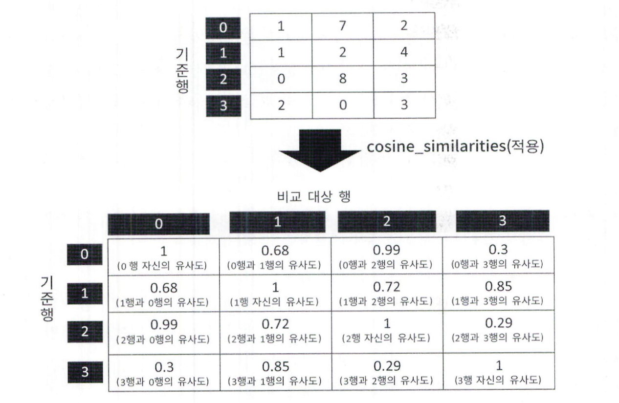
• 이 피처 벡터 행렬을 기반으로 사이킷런의 cosine_similarity() 함수를 사용해 코사인 유사도를 계산

• cosine_similarity() 함수는 기준 행과 비교 행의 코사인 유사도를 계산하여 행렬 형태로 반환

• 이 함수는 각 영화 간 장르 기반 유사도를 수치화해 콘텐츠 기반 필터링 추천 시스템에서 핵심 역할 수행
  

• 피처 벡터화된 행렬에 cosine_similarity() 함수를 적용하여 모든 영화 간의 장르 유사도를 계산

• 이 함수는 4,803 x 4,803 크기의 코사인 유사도 행렬을 반환

• 반환된 행렬에서 앞 2개 데이터(예: 상위 2개 영화 간 유사도)만 추출하여 확인함

from sklearn.metrics.pairwise import cosine_similarity

genre_sim = cosine_similarity(genre_mat, genre_mat)
print(genre_sim.shape)
print(genre_sim[:2])
     

• genre_sim 객체는 genre_literal 칼럼을 CountVectorizer로 벡터화한 결과로,
  각 영화 간 장르 유사도(cosine similarity) 값을 담고 있음
• movies_df의 각 영화(행)별로, 장르 유사도가 높은 다른 영화들의 인덱스를 정렬하여 추출해야 함
• 이를 위해 genre_sim.argsort()[:, ::-1]을 사용함
• argsort()는 유사도 값을 오름차순 정렬한 인덱스를 반환
• [:, ::-1]를 붙이면 내림차순(가장 유사한 영화부터) 정렬
• 예: genre_sim.argsort()[:, ::-1][0] → 0번 영화와 장르 유사도가 높은 순서대로 정렬된 영화 인덱스 리스트 반환

genre_sim_sorted_ind = genre_sim.argsort()[:, ::-1]
print(genre_sim_sorted_ind[:1])

• [[0, 3494, 813, ..., 3038, 3037, 2401]]는 0번 영화의 장르 기준 유사도 정렬 인덱스를 의미함
• 0은 자기 자신이고, 3494번 영화가 유사도 가장 높음 다음은 813,가장 낮은 유사도는 2401번 영화 genre_sim_sorted_ind 객체는 각 영화별로 장르 코사인 유사도가 높은 영화들의 인덱스를 내림차순 정렬한 결과임
• 이를 통해 유사한 영화 추천을 효율적으로 수행할 수 있음

장르 콘텐츠 필터링을 이용한 영화 추천

• 장르 유사도를 기반으로 영화를 추천하는 함수 생성
• 함수 이름: find_sim_movie()
• 입력 인자:
  movies_df: 영화 정보를 담은 DataFrame
  genre_sim_sorted_ind: 각 영화의 장르 유사도 기준 정렬 인덱스
  title_name: 사용자가 기준으로 삼은 영화 제목
  top_n: 추천할 영화 수
• 반환값:
  추천 영화 정보를 담은 DataFrame (장르 유사도 높은 순 정렬)

def find_sim_movie(df, sorted_ind, title_name, top_n=10):

    # 인자로 입력된 movies_df DataFrame에서 'title' 컬럼이 입력된 title_name 값인 DataFrame추출
    title_movie = df[df['title'] == title_name]

    # title_named을 가진 DataFrame의 index 객체를 ndarray로 반환하고
    # sorted_ind 인자로 입력된 genre_sim_sorted_ind 객체에서 유사도 순으로 top_n 개의 index 추출
    title_index = title_movie.index.values
    similar_indexes = sorted_ind[title_index, :(top_n)]

    # 추출된 top_n index들 출력. top_n index는 2차원 데이터 임.
    #dataframe에서 index로 사용하기 위해서 1차원 array로 변경
    print(similar_indexes)
    similar_indexes = similar_indexes.reshape(-1)

    return df.iloc[similar_indexes]
     

find_sim_movie() 함수를 이용해 영화 대부'와 장르 별로 유사한 영화 10개를 추천해 보겠습니다.

similar_movies = find_sim_movie(movies_df, genre_sim_sorted_ind, 'The Godfather',10)
similar_movies[['title', 'vote_average']]

• '대부 2편(The Godfather: Part II)'이 장르 유사도 기반 추천에서 가장 먼저 추천됨
• 유사한 영화로 '좋은 친구들(Goodfellas)'도 포함되어 있음
• 그러나 '라이트 슬리퍼', 'Mi America', 'Kids' 등은 평점이 낮거나 없음 → 추천에 적합하지 않을 수 있음
• 개선 방안:
  유사도 기반으로 더 많은 후보군 확보
  vote_average 기준으로 필터링해 최종 추천
  vote_average는 평균 평점이지만, 평가 인원 수가 적으면 왜곡될 수 있음
• 확인 방법:
  sort_values()로 평점 기준 정렬 후 상위 10개 출력해 데이터 확인

movies_df[['title','vote_average','vote_count']].sort_values('vote_average', ascending=False)[:10]
     

• '쇼생크 탈출(The Shawshank Redemption)', '대부(The Godfather)' 같은 명작보다 생소한 영화들이 더 높은 평점으로 나타남
  예: 'Stiff Upper Lips', 'Me You and Five Bucks' 등 → 이유: 평가 횟수가 매우 적음

• 평점 왜곡 회피 필요 → 평가 횟수를 반영한 새로운 평가 방식 필요

• IMDb에서는 평가 횟수 기반 가중 평점(Weighted Rating) 방식을 사용

• 이 방식을 이용해 새롭게 평점을 부여

$가중 평점 (Weighted Rating) = (v / (v + m)) * R + (m / (v + m)) * C$

• v : 개별 영화에 평점을 투표한 횟수
• m : 평점을 부여하기 위한 최소 투표 횟수
• R : 개별 영화에 대한 평균 평점
• C : 전체 영화에 대한 평균 평점

• v는 각 영화의 'vote_count' 값 (투표 수)
• R은 'vote_average' 값 (평균 평점)
• C는 전체 영화의 평균 평점 → movies_df['vote_average'].mean()
• m은 가중치를 부여하기 위한 기준 투표 수
• m이 높을수록 많은 투표를 받은 영화에 높은 신뢰도 부여
• m은 전체 'vote_count'에서 상위 60%에 해당하는 값으로 설정
• movies_df['vote_count'].quantile(0.6) 로 계산 가능

C = movies_df['vote_average'].mean()
m = movies_df['vote_count'].quantile(0.6)
print('C:',round(C,3), 'm:',round(m,3))

• 기존 평점을 가중 평점으로 변경하기 위해 weighted_vote_average() 함수를 생성함
• 이 함수는 DataFrame의 레코드를 받아 vote_count, vote_average, 미리 구한 m, C 값을 적용해 가중 평점을 계산함
• apply() 함수를 통해 movies_df에 적용하여 vote_weighted 컬럼을 생성함

percentile = 0.6
m = movies_df['vote_count'].quantile(percentile)
C = movies_df['vote_average'].mean()

def weighted_vote_average(record):
    v = record['vote_count']
    R = record['vote_average']

    return ( (v/(v+m)) * R ) + ( (m/(m+v)) * C )

movies_df['weighted_vote'] = movies_df.apply(weighted_vote_average, axis=1)

새롭게 부여된 weighted_vote 평점이 높은 순으로 상위 10개의 영화를 추출해 보겠습니다.

movies_df[['title','vote_average','weighted_vote','vote_count']].sort_values('weighted_vote',
                                                                          ascending=False)[:10]

• 개인의 성향에 따라 TOP 10 영화에 대한 의견 차이는 있을 수 있지만, 추천된 영화들은 모두 뛰어난 작품임
• ‘센과 치히로의 행방불명’의 영어 제목은 Spirited Away임
• 새롭게 정의된 가중 평점을 기준으로 영화를 추천할 계획임
• 장르 유사성이 높은 영화들을 top_n의 2배수만큼 후보로 선정하고, 이들 중 weighted_vote 값이 높은 상위 top_n개의 영화를 추천하도록 find_sim_movie() 함수를 수정함
• 변경된 함수를 이용해 ‘대부’와 유사한 영화들을 콘텐츠 기반 필터링 방식으로 추천함

def find_sim_movie(df, sorted_ind, title_name, top_n=10):
    title_movie = df[df['title'] == title_name]
    title_index = title_movie.index.values

    # top_n의 2배에 해당하는 쟝르 유사성이 높은 index 추출
    similar_indexes = sorted_ind[title_index, :(top_n*2)]
    similar_indexes = similar_indexes.reshape(-1)
# 기준 영화 index는 제외
    similar_indexes = similar_indexes[similar_indexes != title_index]

    # top_n의 2배에 해당하는 후보군에서 weighted_vote 높은 순으로 top_n 만큼 추출
    return df.iloc[similar_indexes].sort_values('weighted_vote', ascending=False)[:top_n]

similar_movies = find_sim_movie(movies_df, genre_sim_sorted_ind, 'The Godfather',10)
similar_movies[['title', 'vote_average', 'weighted_vote']]

• 새로 추천된 영화들은 이전보다 훨씬 우수한 결과를 보임
• 특히 Once Upon a Time in America는 ‘대부’를 좋아하는 사람에게 적절한 추천임
• 그러나 장르만으로는 영화의 분위기나 개인 성향을 충분히 반영하기 어려움
• 실제로는 감독이나 배우에 따라 영화를 선택하는 경우가 많음
• 장르 기반 콘텐츠 필터링을 더 확장할 수 있으나, 이는 과제로 남김
• 다음 단계로 아이템 기반 최근접 이웃 협업 필터링 구현으로 넘어감

6. 아이템 기반 최근접 이웃 협업 필터링 실습

데이터 가공 및 변환

import pandas as pd
import numpy as np

movies = pd.read_csv('/content/sample_data/movies.csv')
ratings = pd.read_csv('/content/sample_data/ratings.csv')
print(movies.shape)
print(ratings.shape)
     

• ratings.csv는 사용자별 영화 평점 데이터로 총 100,836개 레코드로 구성됨
• 주요 컬럼: userId, movieId, rating
• 평점은 0.5 ~ 5.0 사이의 0.5 단위로 부여됨
• timestamp 컬럼은 이번 분석에선 사용하지 않음
• 협업 필터링은 사용자–아이템 간 평점 기반 추천 방식임
• 아이템 기반 최근접 이웃 협업 필터링 구현을 위해
• 원본 데이터셋을 사용자별 row, 영화별 column으로 구성된 형태로 변환해야 함

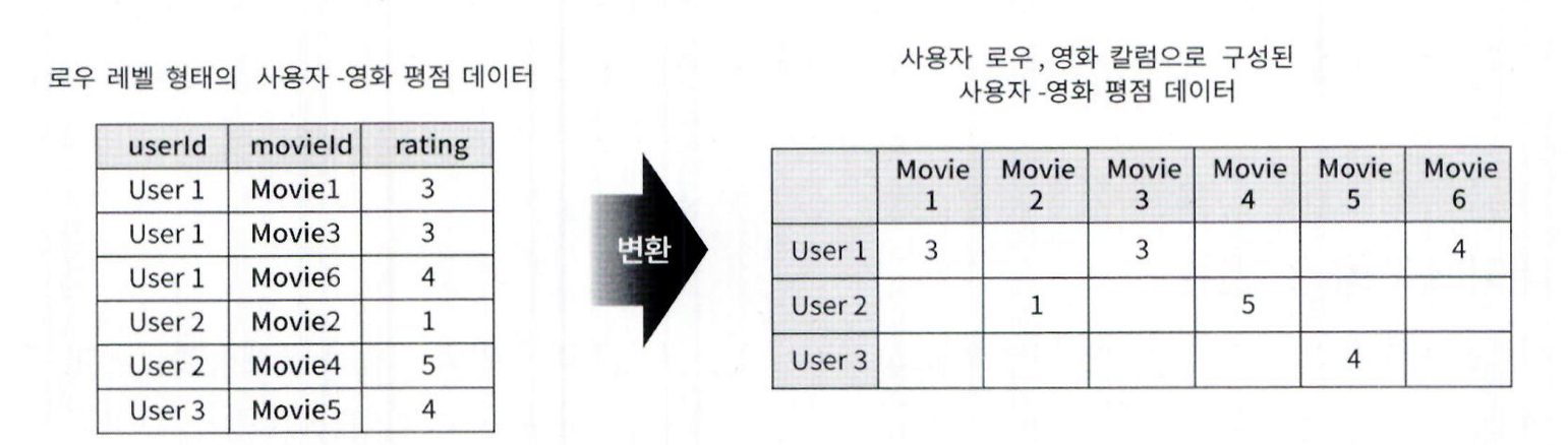
• pivot_table() 함수는 row 형태의 데이터를 column 형태로 쉽게 변환 가능

• columns='movieId'를 지정하면 movieId 값이 새로운 열 이름이 됨

• ratings.pivot_table('rating', index='userId', columns='movieId') 호출 시
  행: userId
  열: movieId
  값: rating

• 즉, 사용자-아이템 평점 행렬로 변환됨

ratings = ratings[['userId', 'movieId', 'rating']]
ratings_matrix = ratings.pivot_table('rating', index='userId', columns='movieId')
ratings_matrix.head(3)
     

• pivot_table()로 만든 평점 행렬에서 movieId는 숫자라 가독성이 떨어짐
• 영화 제목은 ratings에는 없고, movies 데이터셋에 있음
• 따라서 ratings와 movies를 조인(merge)해 title 컬럼을 가져와야 함
• 이후 pivot_table(columns='title')로 영화 제목을 기준으로 피벗 수행
• 사용자-영화 제목 기반 평점 행렬이 생성됨
• 이 행렬에서 NaN 값은 평점을 주지 않은 것으로 간주하고 0으로 변환함

# title 컬럼을 얻기 이해 movies 와 조인 수행
rating_movies = pd.merge(ratings, movies, on='movieId')

# columns='title' 로 title 컬럼으로 pivot 수행.
ratings_matrix = rating_movies.pivot_table('rating', index='userId', columns='title')

# NaN 값을 모두 0 으로 변환
ratings_matrix = ratings_matrix.fillna(0)
ratings_matrix.head(3)
     

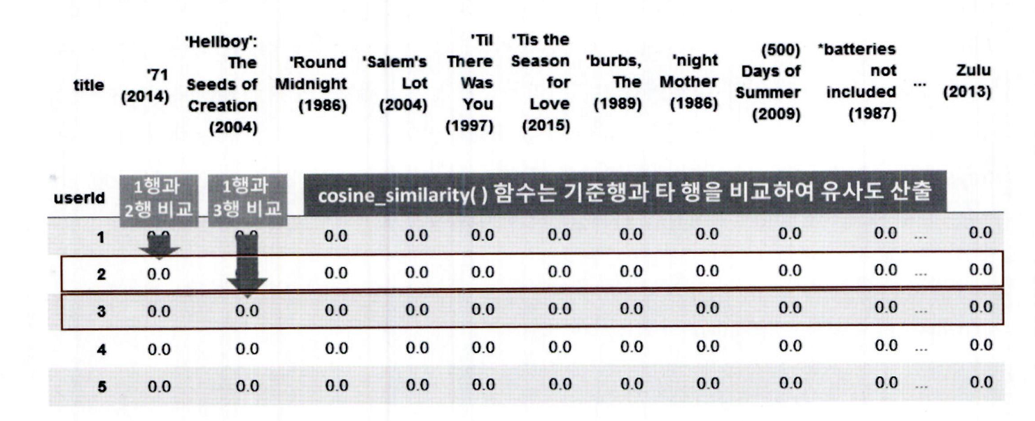
영화 간 유사도 산출

• ratings_matrix는 현재 사용자(userId)를 행, 영화(title)를 열로 구성함
• 하지만 cosine_similarity()는 행 간 유사도를 계산하므로, 현재 상태로는 사용자 간 유사도가 나옴
• 영화 간 유사도를 계산하려면 행을 영화로 바꿔야 함
• 따라서 ratings_matrix.transpose()를 적용해 행: 영화, 열: 사용자 구조로 변환함
• 이렇게 변환된 행렬에 cosine_similarity()를 적용하면 영화 간 유사도 행렬이 생성됨

ratings_matrix_T = ratings_matrix.transpose()
ratings_matrix_T.head(3)

ratings_matrix 를 전치 행렬 형식으로 변경한 데이터셋을 기반으로 영화의 코사인 유사도를 구해보겠습니다.

그리고 좀 더 직관적인 영화의 유사도 값을 표현하기 위해 cosine_similarity() 로 반환된 넘파이 행렬에 영화명을 매핑해 DataFrame 으로 변환하겠습니다.

from sklearn.metrics.pairwise import cosine_similarity

item_sim = cosine_similarity(ratings_matrix_T, ratings_matrix_T)

# cosine_similarity() 로 반환된 넘파이 행렬을 영화명을 매핑하여 DataFrame으로 변환
item_sim_df = pd.DataFrame(data=item_sim, index=ratings_matrix.columns,
                          columns=ratings_matrix.columns)
print(item_sim_df.shape)
item_sim_df.head(3)

7. 행렬 분해를 이용한 잠재 요인 협업 필터링 실습

• 확률적 경사 하강법(SGD)을 이용해 사용자–아이템 평점 행렬을 행렬 분해(Matrix Factorization) 하여, 추천 시스템을 구현

• R: 원본 평점 행렬 (사용자 × 아이템)

• K: 잠재 요인 수

• steps: 반복 횟수

• learning_rate: 학습률

• r_lambda: L2 정규화 계수

• 구현:
  get_rmse(): 예측 평점과 실제 평점의 RMSE 계산 함수
  matrix_factorization(): 위 파라미터로 행렬 분해를 수행하는 함수로 정의하여 재사용 가능하게 구성

# Uninstall existing scikit-surprise and numpy to ensure a clean installation
!pip uninstall scikit-surprise numpy -y

# Install a compatible version of numpy first
!pip install numpy==1.24.4 # You can try a different version if this doesn't work

# Reinstall scikit-surprise
!pip install scikit-surprise

# Import surprise again to check if the error is resolved
import surprise

print(surprise.__version__)

# Also check the numpy version
import numpy
print(numpy.__version__)

import surprise

print(surprise.__version__)

!pip uninstall scikit-surprise numpy -y

# Install a compatible version of numpy first. Use a version known to work well with surprise.
# numpy==1.24.4 is a good starting point.
!pip install numpy==1.24.4

# Reinstall scikit-surprise
!pip install scikit-surprise

# Import surprise again to check if the error is resolved
import surprise

print(surprise.__version__)

# Also check the numpy version
import numpy
print(numpy.__version__)

# Import the required modules from surprise
from surprise import SVD
from surprise import Dataset
from surprise import accuracy
from surprise.model_selection import train_test_split

!pip uninstall numpy -y
!pip install numpy
     

# Import the required modules from surprise
from surprise import SVD
from surprise import Dataset
from surprise import accuracy
from surprise.model_selection import train_test_split

# Load the built-in dataset
data = Dataset.load_builtin('ml-100k')

# Split the data into training and testing sets for reproducibility
trainset, testset = train_test_split(data, test_size=.25, random_state=0)

algo = SVD(random_state=0)
algo.fit(trainset)

predictions = algo.test( testset )
print('prediction type :',type(predictions), ' size:',len(predictions))
print('prediction 결과의 최초 5개 추출')
predictions[:5]

[ (pred.uid, pred.iid, pred.est) for pred in predictions[:3] ]

# 사용자 아이디, 아이템 아이디는 문자열로 입력해야 함.
uid = str(196)
iid = str(302)
pred = algo.predict(uid, iid)
print(pred)

accuracy.rmse(predictions)

import pandas as pd

ratings = pd.read_csv('/content/sample_data/ratings.csv')
# ratings_noh.csv 파일로 unload 시 index 와 header를 모두 제거한 새로운 파일 생성.
ratings.to_csv('/content/sample_data/ratings_noh.csv', index=False, header=False)

from surprise import Reader

reader = Reader(line_format='user item rating timestamp', sep=',', rating_scale=(0.5, 5))
data=Dataset.load_from_file('/content/sample_data/ratings_noh.csv',reader=reader)
     

trainset, testset = train_test_split(data, test_size=.25, random_state=0)

# 수행시마다 동일한 결과 도출을 위해 random_state 설정
algo = SVD(n_factors=50, random_state=0)

# 학습 데이터 세트로 학습 후 테스트 데이터 세트로 평점 예측 후 RMSE 평가
algo.fit(trainset)
predictions = algo.test( testset )
accuracy.rmse(predictions)

import pandas as pd
from surprise import Reader, Dataset

ratings = pd.read_csv('/content/sample_data/ratings.csv')
reader = Reader(rating_scale=(0.5, 5.0))

# ratings DataFrame 에서 컬럼은 사용자 아이디, 아이템 아이디, 평점 순서를 지켜야 합니다.
data = Dataset.load_from_df(ratings[['userId', 'movieId', 'rating']], reader)
trainset, testset = train_test_split(data, test_size=.25, random_state=0)

algo = SVD(n_factors=50, random_state=0)
algo.fit(trainset)
predictions = algo.test( testset )
accuracy.rmse(predictions)
     

from surprise.model_selection import cross_validate

# 판다스 DataFrame에서 Surprise 데이터 세트로 데이터 로딩
ratings = pd.read_csv('/content/sample_data/ratings.csv') # reading data in pandas df
reader = Reader(rating_scale=(0.5, 5.0))
data = Dataset.load_from_df(ratings[['userId', 'movieId', 'rating']], reader)

algo = SVD(random_state=0)
cross_validate(algo, data, measures=['RMSE', 'MAE'], cv=5, verbose=True)
     

from surprise.model_selection import GridSearchCV

# 최적화할 파라미터를 딕셔너리 형태로 지정.
param_grid = {'n_epochs': [20, 40, 60], 'n_factors': [50, 100, 200] }

# CV를 3개 폴드 세트로 지정, 성능 평가는 rmse, mse로 수행하도록 GridSearchCV 구성
gs = GridSearchCV(SVD, param_grid, measures=['rmse', 'mae'], cv=3)
gs.fit(data)

# 최고 RMSE Evaluation 점수와 그때의 하이퍼 파라미터
print(gs.best_score['rmse'])
print(gs.best_params['rmse'])
     

from surprise.dataset import DatasetAutoFolds

reader = Reader(line_format='user item rating timestamp', sep=',', rating_scale=(0.5, 5))
# DatasetAutoFolds 클래스를 ratings_noh.csv 파일 기반으로 생성.
data_folds = DatasetAutoFolds(ratings_file='/content/sample_data/ratings_noh.csv', reader=reader)

#전체 데이터를 학습데이터로 생성함.
trainset = data_folds.build_full_trainset()

algo = SVD(n_epochs=20, n_factors=50, random_state=0)
algo.fit(trainset)
     

# 영화에 대한 상세 속성 정보 DataFrame로딩
movies = pd.read_csv('/content/sample_data/movies.csv')

# userId=9 의 movieId 데이터 추출하여 movieId=42 데이터가 있는지 확인.
movieIds = ratings[ratings['userId']==9]['movieId']
if movieIds[movieIds==42].count() == 0:
    print('사용자 아이디 9는 영화 아이디 42의 평점 없음')

print(movies[movies['movieId']==42])

uid = str(9)
iid = str(42)

pred = algo.predict(uid, iid, verbose=True)
     

def get_unseen_surprise(ratings, movies, userId):
    #입력값으로 들어온 userId에 해당하는 사용자가 평점을 매긴 모든 영화를 리스트로 생성
    seen_movies = ratings[ratings['userId']== userId]['movieId'].tolist()

    # 모든 영화들의 movieId를 리스트로 생성.
    total_movies = movies['movieId'].tolist()

    # 모든 영화들의 movieId중 이미 평점을 매긴 영화의 movieId를 제외하여 리스트로 생성
    unseen_movies= [movie for movie in total_movies if movie not in seen_movies]
    print('평점 매긴 영화수:',len(seen_movies), '추천대상 영화수:',len(unseen_movies), \
          '전체 영화수:',len(total_movies))

    return unseen_movies

unseen_movies = get_unseen_surprise(ratings, movies, 9)
     

def recomm_movie_by_surprise(algo, userId, unseen_movies, top_n=10):
    # 알고리즘 객체의 predict() 메서드를 평점이 없는 영화에 반복 수행한 후 결과를 list 객체로 저장
    predictions = [algo.predict(str(userId), str(movieId)) for movieId in unseen_movies]

    # predictions list 객체는 surprise의 Predictions 객체를 원소로 가지고 있음.
    # [Prediction(uid='9', iid='1', est=3.69), Prediction(uid='9', iid='2', est=2.98),,,,]
    # 이를 est 값으로 정렬하기 위해서 아래의 sortkey_est 함수를 정의함.
    # sortkey_est 함수는 list 객체의 sort() 함수의 키 값으로 사용되어 정렬 수행.
    def sortkey_est(pred):
        return pred.est

    # sortkey_est( ) 반환값의 내림 차순으로 정렬 수행하고 top_n개의 최상위 값 추출.
    predictions.sort(key=sortkey_est, reverse=True)
    top_predictions= predictions[:top_n]

    # top_n으로 추출된 영화의 정보 추출. 영화 아이디, 추천 예상 평점, 제목 추출
    top_movie_ids = [ int(pred.iid) for pred in top_predictions]
    top_movie_rating = [ pred.est for pred in top_predictions]
    top_movie_titles = movies[movies.movieId.isin(top_movie_ids)]['title']
    top_movie_preds = [ (id, title, rating) for id, title, rating in zip(top_movie_ids, top_movie_titles, top_movie_rating)]

    return top_movie_preds

unseen_movies = get_unseen_surprise(ratings, movies, 9)
top_movie_preds = recomm_movie_by_surprise(algo, 9, unseen_movies, top_n=10)
print('##### Top-10 추천 영화 리스트 #####')

for top_movie in top_movie_preds:
    print(top_movie[1], ":", top_movie[2])