https://github.com/nalinzip/ml_study/blob/main/ML_Week11.ipynb

1. NLP 이냐 텍스트 분석이냐?

• NLP 는 머신이 인간의 언어를 이해하고 해석하는 데 더 중점을 두고 기술이 발전해 왔음

• 텍스트 마이닝 (Text Mining) 이라고도 불리는 텍스트 분석 (Text Analytics, 이하 TA) 은 비정형 텍스트에서 의미 있는 정보를 추출하는 것에 좀 더 중점을 두고 기술이 발전해 왔음

• 예를 들어 NLP 의 영역에는 언어를 해석하기 위한 기계 번역 , 자동으로 질문을 해석하고 답을 해주는 질의응답 시스템 등의 영역 등에서 텍스트 분석과 차별점이 있음

• NLP 는 텍스트 분석을 향상하게 하는 기반 기술이라고 볼 수도 있음

• NLP 기술이 발전함에 따라 텍스트 분석도 더욱 정교하게 발
  전할 수 있었음

• NLP 와 텍스트 분석의 발전 근간에는 머신러닝이 존재함

• 예전의 텍스트를 구성하는 언어적인 룰이나 업무의 룰에 따라 텍스트를 분석하는 룰 기반 시스템에서 머신러닝의 텍스트 데이터를 기반으로 모델을 학습하고 예측하는 기반으로 변경되면서 많은 기술적 발전이 가능해졌음

• 텍스트 분석은 머신러닝 , 언어 이해 , 통계 등을 활용해 모델을 수립하고 정보를 추출해 비즈니스 인텔리전스 (Business Intelligence)나 예측 분석 등의 분석 작업을 주로 수행함

• 머신러닝 기술에 힘입어 텍스트 분석은 크게 발전하고 있음

주로 다음과 같은 기술 영역에 집중

텍스트 분류 (Text Classification) / Text Categorization

• 문서가 특정 분류 또는 카테고리에 속하는 것을 예측하는 기법을 통칭함
• 예를 들어 특정 신문 기사 내용이 연예 / 정치 / 사회 / 문화 중 어떤 카테고리에 속하는지 자동으로 분류하거나 스팸 메일 검출 같은 프로그램이 이에 속함
• 지도학습을 적용함

감성 분석(Sentiment Analysis)

• 텍스트에서 나타나는 감정 / 판단 / 믿음 / 의견 / 기분 등의 주관적인 요소를 분석하는 기법을 총칭함
• 소셜 미디어 감정 분석 , 영화나 제품에 대한 긍정 또는 리뷰 , 여론조사 의견 분석 등의 다양한 영역에서 활용됨
• Text Analytics 에서 가장 활발하게 사용되고 있는 분야임
• 지도학습 방법뿐만 아니라 비지도 학습을 이용해 적용할 수 있음

텍스트 요약 (Summarization)

• 텍스트 내에서 중요한 주제나 중심 사상을 추출하는 기법을 말함
• 대표적으로 토픽 모델링 (Topic Modeling)

텍스트 군집화 (Clustering) 와 유사도 측정

• 비슷한 유형의 문서에 대해 군집화를 수행하는 기법을 말함
• 텍스트 분류를 비지도학습으로 수행하는 방법의 일환으로 사용될 수 있습니다. 유사도 측정 역시 문서들간의 유사도를 측정해 비슷한 문서끼리 모을 수 있는 방법임

텍스트 분석 이해

• 텍스트 분석은 비정형 데이터인 텍스트를 분석하는 것임
• 지금까지 ML 모델은 주어진 정형 데이터 기반에서 모델을 수립하고 예측을 수행했음
• 그리고 머신러닝 알고리즘은 숫자형의 피처 기반 데이터만 입력받을 수 있기 때문에 텍스트를 머신러닝에 적용하기 위해서는 비정형 텍스트 데이터를 어떻게 피처 형태로 추출하고 추출된 피처에 의미 있는 값을 부여하는가 하는 것이 매우 중요한 요소임
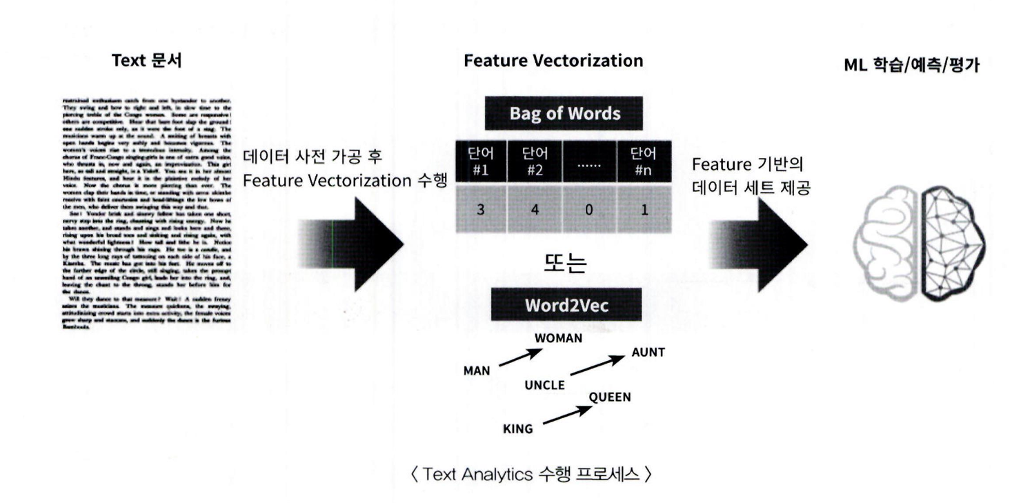
• 텍스트를 word( 또는 word 의 일부분 ) 기반의 다수의 피처로 추출하고 이 피처에 단어 빈도수와 같은 숫자 값을 부여하면 텍스트는 단어의 조합인 벡터값으로 표현될 수 있는데, 이렇게 텍스트를 변환하는 것을 피처 벡터화 (Feature Vectorization) 또는 피처 추출 (Feature Extraction) 이라고 함
• 대표적으로 텍스트를 피처 벡터화해서 변환하는 방법에는 BOW(Bag of Words) 와 Word2Vec 방법이 있음
• 텍스트를 벡터값을 가지는 피처로 변환하는 것은 머신러닝 모델을 적용하기 전에 수행해야 할 매우 중요한 요소입임
  

텍스트 분석 수행 프로세스

머신러닝 기반의 텍스트 분석 프로세스

1. 텍스트 사전 준비작업 ( 텍스트 전처리 ): 텍스트를 피처로 만들기 전에 미리 클렌징 , 대 / 소문자 변경 , 특수문자 삭제
   등의 클렌징 작업 , 단어 (Word) 등의 토큰화 작업 , 의미 없는 단어 (Stop Word) 제거 작업 , 어근 추출 (Stemming/Lemmatization) 등의 텍스트 정규화 작업을 수행하는 것을 통칭합니다.
2. 피처 벡터화 / 추출: 사전 준비 작업으로 가공된 텍스트에서 피처를 추출하고 여기에 벡터 값을 할당합니다. 대표적
   인 방법은 BOW 와 WordeVec이 있으며 , BOW 는 대표적으로 Count 기반과 TF-DF 기반 벡터화가 있습니다.
3. ML 모델 수립 및 학습 / 예측 / 평가 : 피처 벡터화된 데이터 세트에 ML 모델을 적용해 학습 / 예측 및 평가를 수행합
   니다.

파이썬 기반의 NLP, 텍스트 분석 패키지

• 파이썬 기반에서 NLP 와 텍스트 분석을 위해 쉽고 편하게 텍스트 사전 정제 작업 , 피처 벡터화 / 추출 , ML 모델을 지원하는 매우 훌륭한 라이브러리가 많음
• 대표적인 파이썬 기반의 NIP 와 텍스트 분석 패키지를 소개함

• NLTK 는 방대한 데이터 세트와 서브 모듈, 다양한 데이터 세트를 지원해 오래전부터 대표적인 파이썬 NLP 패키지였지만 , 수행 성능과 정확도 , 신기술 , 엔터프라이즈한 기능 지원 등의 측면에서 부족한 부분이 있음
• Genism 과 SpaCy 는 이러한 부분을 보완하면서 실제 업무에서 자주 활용되는 패키지임

NLTK(Natural Language Toolkit for Python)

• 파이썬의 가장 대표적인 NLP 패키지
• 방대한 데이터 세트와 서브 모듈을 가지고 있으며 NLP 의 거의 모든 영역을 커버하고 있음
• 많은 NLP 패키지가 NLTK 의 영향을 받아 작성되고 있음
• 수행 속도 측면에서 아쉬운 부분이 있어서 실제 대량의 데이터 기반에서는 제대로 활용되지 못하고 있음

Gensim

• 토픽 모델링 분야에서 가장 두각을 나타내는 패키지입니다. 오래전부터 토픽 모델링을 쉽게 구현할 수 있는 기능을 제공해 왔으며 , WordeVec 구현 등의 다양한 신기능도 제공함
• SpaCy 와 함께 가장 많이 사용되는 NLP 패키지임

SpaCy

• 뛰어난 수행 성능으로 최근 가장 주목을 받는 NLP 패키지임
• 많은 NLP 애플리케이션에서 SpaCy 를 사용하는 사례가 늘고 있음

• 사이킷런은 머신러닝 중심의 라이브러리로, NLP에 특화된 기능은 제한적임.

• 하지만 텍스트 전처리 및 머신러닝 모델 입력을 위한 기본적인 텍스트 가공 및 피처 처리 기능은 제공함.

• 복잡한 NLP 작업이 필요한 경우에는 NLTK, Gensim, SpaCy 등의 NLP 전용 라이브러리와 함께 사용함.

2. 텍스트 사전 준비 작업 ( 텍스트 전처리 ) - 텍스트 정규화

• 텍스트 자체를 바로 피처로 만들 수는 없기 때문에 사전에 텍스트를 가공하는 준비 작업이 필요함
• 텍스트 정규화는 텍스트를 머신러닝 알고리즘이나 NLP 애플리케이션에 입력 데이터로 사용하기 위해 클렌징, 정제, 토큰화, 어근 등의 다양한 텍스트 데이터의 사전 작업을 수행하는 것을 의미함 - 텍스트 분석은 이러한 텍스트 정규화 작업이 매우 중요함

텍스트 정규화 작업 분류

1. 클렌징 (Cleansing)
   텍스트에서 분석에 오히려 방해가 되는 불필요한 문자 , 기호 등을 사전에 제거하는 작업임
   예를 들어 HTML, XML 태그나 특정 기호 등을 사전에 제거함
2. 토큰화 (Tokenization)
3. 필터링 / 스톱 워드 제거 / 철자 수정
4. Stemming
5. Lemmatization

텍스트 토큰화

• 토큰화의 유형은 문서에서 문장을 분리하는 문장 토큰화와 문장에서 단어를 토큰으로 분리하는 단어 토큰화로 나눌 수 있음
• NLTK 는 이를 위해 다양한 API 를 제공

문장 토큰화

• 문장 토큰화 (sentence tokenization) 는 문장의 마침표 (.), 개행문자 (\n) 등 문장의 마지막을 뜻하는 기호에 따라 분리하는 것이 일반적임

• 또한 정규 표현식에 따른 문장 토큰화도 가능

• NTLK에서 일반적으로 많이 쓰이는 sent_tokenize 를 이용해 토큰화 수행

• 다음은 3 개의 문장으로 이루어진 텍스트 문서를 문장으로 각각 분리하는 예제

• NLTK 의 경우 단어 사전과 같이참조가 필요한 데이터 세트의 경우 인터넷으로 다운로드받을 수 있음

• 다운로드가 완료된 경우에는 다시 다운로드하지 않지만 최초 다운로드가 필요하기 때문에 수행하려는 컴퓨터에 인터넷 연결이 돼 있는지 먼저 확인하고 다운로드를 수행하면 됨

• nltk.download('punkt')는 마침표 , 개행 문자등의 데이터 세트를 다운로드함

from nltk import sent_tokenize
import nltk

nltk.download('punkt')

text_sample = 'The Matrix is everywhere its all around us, here even in this room. \
               You can see it out your window or on your television. \
               You feel it when you go to work, or go to church or pay your taxes.'
sentences = sent_tokenize(text=text_sample)
print(type(sentences),len(sentences))
print(sentences)

• sent_tokenize()가 반환하는 것은 각각의 문장으로 구성된 list 객체임
• 반환된 list 객체가 3 개의 문장으로 된 문자열을 가지고 있는 것을 알 수 있음

단어 토큰화

• 단어 토큰화 (Word Tokenization)는 문장을 단어로 토큰화하는 것
• 기본적으로 공백 , 콤마 (,). 마침표 (.), 개행문자 등으로 단어를 분리하지만 , 정규 표현식을 이용해 다양한 유형으로 토큰화를 수행할 수 있음
• 마침표 (.) 나 개행문자와 같이 문장을 분리하는 구분자를 이용해 단어를 토큰화할 수 있으므로 Bag ofWord 와 같이 단어의 순서가 중요하지 않은 경우 문장 토큰화를 사용하지 않고 단어 토큰화만 사용해도 충분
• 일반적으로 문장 토큰화는 각 문장이 가지는 시맨틱적인 의미가 중요한 요소로 사용될 때 사용함

NTLK 에서 기본으로 제공하는 word_tokenize() 를 이용해 단어로 토큰화

from nltk import word_tokenize

sentence = "The Matrix is everywhere its all around us, here even in this room."
words = word_tokenize(sentence)
print(type(words), len(words))
print(words)

sent_tokenize 와 word_tokenize를 조합해 문서에 대해서 모든 단어를 토큰화해

문서를 먼저 문장으로 나누고 , 개별 문장을 다시 단어로 토큰화하는 tokenize_text() 함수를 생성

from nltk import word_tokenize, sent_tokenize

#여러개의 문장으로 된 입력 데이터를 문장별로 단어 토큰화 만드는 함수 생성
def tokenize_text(text):
    
    # 문장별로 분리 토큰
    sentences = sent_tokenize(text)
    # 분리된 문장별 단어 토큰화
    word_tokens = [word_tokenize(sentence) for sentence in sentences]
    return word_tokens

#여러 문장들에 대해 문장별 단어 토큰화 수행. 
word_tokens = tokenize_text(text_sample)
print(type(word_tokens),len(word_tokens))
print(word_tokens)

• word_tokens 변수는 3 개의 리스트 객체를 내포하는 리스트임
• 내포된 개별 리스트 객체는 각각 문장별로 토큰화된 단어를 요소로 가지고 있음
• 문장을 단어별로 하나씩 토큰화 할 경우 문맥적인 의미는 무시될 수밖에 없음
• 이러한 문제를 조금이라도 해결해 보고자 도입된 것이 n-gram 임
• n-gram 은 연속된 n 개의 단어를 하나의 토큰화 단위로 분리해 내는 것임
• n 개 단어 크기 윈도우를 만들어 문장의 처음부터 오른쪽으로 움직이면서 토큰화를 수행함
• 예를 들어 "Agent Smith knocks the door" 를 2-gram(bigram) 으로 만들면 → (Agent, Smith), (Smith, knocks), (knocks, the), (the, door)와 같이 연속적으로 2 개의 단어들을 순차적으로 이동하면서 단어들을 토큰화 함

스톱 워드 제거

• 스톱 워드 (Stop word) 는 분석에 큰 의미가 없는 단어를 지칭함.
• 가령 영어에서 is, the, a, wil 등 문장을 구성하는 필수 문법 요소지만 문맥적으로 큰 의미가 없는 단어가 이에 해당함
• 이 단어의 경우 문법적인 특성으로 인해 특히 빈번하게 텍스트에 나타나므로 이것들을 사전에 제거하지 않으면 그 빈번함으로 인해 오히려 중요한 단어로 인지될 수 있음
• 따라서 이 의미 없는 단어를 제거하는 것이 중요한 전처리 작업임
• 언어별로 이러한 스톱 워드가 목록화돼 있음.
• NLTK 의 경우 가장 다양한 언어의 스톱 워드를 제공함

---

NTLK 의 스톱 워드에는 어떤 것이 있는지 확인
이를 위해 먼저 NLTK 의 stopwords 목록을 내려받습니다.

import nltk
nltk.download('stopwords')

다운로드가 완료되고 나면 NTLK 의 English의 경우 몇 개의 stopwords가 있는지 알아보고 그중 20개만 확인

print('영어 stop words 갯수:',len(nltk.corpus.stopwords.words('english')))
print(nltk.corpus.stopwords.words('english')[:20])

• 영어의 경우 스톱 워드의 개수가 179 개이며 , 그중 20 개만 살펴보면 위의 결과와 같음

---

문장별로 단어를 토큰화해 생성된 word_tokens 리스트 (3 개의 문장별 단어 토큰화 값을 가지는 내포된 리스트로 구성 )에 대해서 stopwords를 필터링으로 제거해 분석을 위한 의미 있는 단어만 추출

import nltk

stopwords = nltk.corpus.stopwords.words('english')
all_tokens = []
# 위 예제의 3개의 문장별로 얻은 word_tokens list 에 대해 stop word 제거 Loop
for sentence in word_tokens:
    filtered_words=[]
    # 개별 문장별로 tokenize된 sentence list에 대해 stop word 제거 Loop
    for word in sentence:
        #소문자로 모두 변환합니다. 
        word = word.lower()
        # tokenize 된 개별 word가 stop words 들의 단어에 포함되지 않으면 word_tokens에 추가
        if word not in stopwords:
            filtered_words.append(word)
    all_tokens.append(filtered_words)
    
print(all_tokens)

is, this 와 같은 스톱 워드가 필터링을 통해 제거됐음

Stemming Lemmatization

• 많은 언어에서 문법적인 요소에 따라 단어가 다양하게 변함
• 영어의 경우 과거 / 현재 , 3 인칭 단수 여부 , 진행형 등 매우 많은 조건에 따라 원래 단어가 변화함
• 가령 work 는 동사 원형인 단어지만 , 과거형은 worked, 3 인칭 단수일 때 works, 진행형인 경우 Working 등 다양하게 달라짐
• Stemming 과 Lemmatization 은 문법적 또는 의미적으로 변화하는 단어의 원형을 찾는 것임
• 두 기능 모두 원형 단어를 찾는다는 목적은 유사하지만 , Lemmatization이 Stemming 보다 정교하며 의미론적인 기반에서 단어의 원형을 찾음
• Stemming 은 원형 단어로 변환 시 일반적인 방법을 적용하거나 더 단순화된 방법을 적용해 원래 단어에서 일부 철자가 훼손된 어근 단어를 추출하는 경향이 있음
• 이에 반해 Lemmatization은 품사와 같은 문법적인 요소와 더 의미적인 부분을 감안해 정확한 철자로 된 어 단어를 찾아줌
• 따라서 Lemmatization이 Stemming 보다 변환에 더 오랜 시간을 필요로 함
• NLTK 는 다양한 Stemmer 를 제공함
• 대표적으로 Porter, Lancaster, Snowball Stemmer가 있음
• 그리고 Lemmatization을 위해서는 WordNetLemmatizer를 제공함

---

Stemming과 Lemmatization을 비교

• 먼저 NLTK 의 LancasterStemmer를 이용해 Stemmer 부터 살펴보기
• 진행형 , 3 인칭 단수 , 과거형에 따른 동사 , 그리고 비교 , 최상에 따른 형용사의 변화에 따라 Stemming은 더 단순하게 원형 단어를 찾아줌
• NTLK 에서는 LancasterStemmer()와 같이 필요한 Stemmer 객체를 생성한 뒤 이 객체의 stem(' 단어 ') 메서드를 호출하면 원하는 단어의 Stemming이 가능함

from nltk.stem import LancasterStemmer
stemmer = LancasterStemmer()

print(stemmer.stem('working'),stemmer.stem('works'),stemmer.stem('worked'))
print(stemmer.stem('amusing'),stemmer.stem('amuses'),stemmer.stem('amused'))
print(stemmer.stem('happier'),stemmer.stem('happiest'))
print(stemmer.stem('fancier'),stemmer.stem('fanciest'))

• work 의 경우 진행형 (working), 3 인칭 단수 (Works), 과거형 (worked) 모두 기본 단어인 Work 에 ing, s, ed 가 불는 단순한 변화이므로 원형 단어로 work 를 제대로 인식
• 하지만 amuse 의 경우 , 각 변화가 amuse 가 아닌 amus 에 ing, s, ed 가 붙으므로 정확한 단어인 amuse 가 아닌 amus 를 원형단어로 인식
• 형용사인 happy, fancy 의 경우도 비교형 , 최상급형으로 변형된 단어의 정확한 원형을 찾지 못하고 원형 단어에서 철자가 다른 어근 단어로 인식하는 경우가 발생함

---

WordNetLemmatizer를 이용해 Lemmatization을 수행

• 일반적으로 Lemmatization 은 보다 정확한 원형 단어 추출을 위해 단어의 품사를 입력해줘야 함
  -lemmatize()의 파라미터로 동사의 경우 'v', 형용사의 경우 'a' 를 입력함

from nltk.stem import WordNetLemmatizer
import nltk
nltk.download('wordnet')

lemma = WordNetLemmatizer()
print(lemma.lemmatize('amusing','v'),lemma.lemmatize('amuses','v'),lemma.lemmatize('amused','v'))
print(lemma.lemmatize('happier','a'),lemma.lemmatize('happiest','a'))
print(lemma.lemmatize('fancier','a'),lemma.lemmatize('fanciest','a'))

stemmer 보다 정확하게 원형 단어를 추출해줌

3. Bag of Words - BOW

Bag of Words 모델은 문서가 가지는 모든 단어 (Words) 를 - 문맥이나 순서를 무시하고 일괄적으로 단어에 대해 빈도 값을 부여해 피처 값을 추출하는 모델입니다. 문서 내 모든 단어를 한꺼번에 봉투 (Bag) 안에 넣은 뒤에 흔들어서 섞는 것이다.

문장을 Bag of words 의 단어 수 (Word Count) 기반으
로 피처를 추출

1. My wife likes to watch baseball games and my daughter likes to watch baseball games too

2. My wife likes to play baseball

3. 문장 1 과 문장 2 에 있는 모든 단어에서 중복을 제거하고 각 단어 (feature 또는 term) 를 칼럼 형태로 나열합니다. 그
   러고 나서 각 단어에 고유의 인덱스를 다음과 같이 부여합니다.
   'and':0, 'baseball': 1, 'daughter': 2, 'games': 3, 'likes':4, 'my':5, 'play': 6, 'to': 7, 'too': 8,'watch': 9, 'wife': 10

4. 개별 문장에서 해당 단어가 나타나는 횟수 (Occurrence) 를 각 단어 ( 단어 인덱스 ) 에 기재합니다. 예를 들어 base-
   bal 은 문장 1, 2 에서 총 2 번 나타나며 , daughter는 문장 1 에서만 1 번 나타납니다.

장점:

• BOW(Bag of Words)는 쉽고 빠르게 구축 가능
• 단어 발생 횟수 기반이지만 문서 특징을 잘 반영함
• 전통적으로 다양한 분야에서 활용도 높음

단점:

• 문맥 의미 부족 (Semantic Context)
• 단어 순서를 고려하지 않아 문맥적인 의미 무시됨
• n-gram으로 보완 가능하나 한계 존재
• 희소 행렬 문제 (Sparsity / Sparse Matrix)
• 단어 수가 많고 대부분 문서에는 일부 단어만 포함됨
• 대부분의 값이 0으로 채워진 희소 행렬 발생
• 희소 행렬은 ML 알고리즘의 성능과 속도 저하시킴
• 별도 희소 행렬 처리 기법 필요
• 밀집 행렬(Dense Matrix)은 대부분 의미 있는 값으로 채워짐

BOW 피처 벡터화

• 머신러닝 알고리즘은 숫자형 피처만 입력 가능 → 텍스트는 벡터로 변환 필요
• 이 변환을 피처 벡터화 (Feature Vectorization) 라고 함
• 예: 각 문서(Document)의 텍스트를 단어로 추출 → 각 단어를 피처로 할당 → 발생 빈도 등을 값으로 부여
• 결과적으로 문서를 단어 피처의 발생 빈도 벡터로 표현
• 텍스트 → 숫자 피처 조합 → 피처 추출의 일종 (Text Analysis에서 동일 개념으로 사용됨)
• BOW 기반 벡터화:
  모든 문서의 단어를 열(칼럼)로 나열
  각 문서에서 단어의 횟수 또는 정규화된 빈도를 값으로 할당
  문서 수 = M, 단어 수 = N → 결과는 M × N 크기의 벡터 형태 데이터셋

일반적으로 BOW 의 피처 벡터화는 두 가지 방식이 있습니다.

• 카운트 기반의 벡터화
• TF-DF(Term Frequency - Inverse Document Frequency) 기반의 벡터화

---

카운트 벡터화 (Count Vectorization):

• 각 문서에서 단어 등장 횟수(Count)를 피처 값으로 부여
• 횟수 높을수록 중요한 단어로 간주됨
• 단점: 자주 사용되는 일반 단어도 높은 값 → 문서 특징 왜곡

TF-IDF 벡터화 (Term Frequency-Inverse Document Frequency):

• 특정 문서에서 자주 나타나는 단어 → 가중치 높음
• 여러 문서에서 반복적으로 등장하는 단어 → 가중치 낮춤 (페널티)
• 예: '분쟁', '유혈 사태' → 특정 주제 문서를 잘 표현 → 가중치↑
  '조직', '당연히' 등 일반 단어 → 여러 문서에 흔히 등장 → 가중치↓

• 카운트 벡터화는 빈도만 고려 → 일반 단어도 중요 단어로 착각
• TF-IDF는 문서별, 전체 문서의 빈도 균형 고려
• 문서 길이 많고 문서 수 클수록 TF-IDF가 더 효과적

Count 및 TF-IDF : CountVectorizer, TfidfVectorizer

• CountVectorizer는 사이킷런에서 제공하는 카운트 기반 벡터화 클래스입니다.
• 이 클래스는 단순히 단어 개수만 세는 것이 아니라 다음과 같은 텍스트 전처리 기능도 함께 수행
  소문자 변환
  토큰화 (단어 단위 분리)
  스톱워드 제거 (의미 없는 단어 필터링 등)
• 사용 방식은 다른 변환기와 동일하게 다음 두 단계로 진행됩니다:
  fit(): 학습 데이터로 어휘 사전 구축
  transform(): 실제 벡터화 수행

주요 특징

• 단어 수 기반 피처 추출
• 전처리 기능 포함
• 머신러닝 입력용으로 적합한 희소 행렬(sparse matrix) 반환

CountVectorizer 주요 입력 파라미터

• stop_words='english': 영어 스톱워드 필터링 가능 (다른 언어는 미지원)
• tokenizer: 사용자 정의 토큰화/어근변환 함수 지정 가능 (Stemming, Lemmatization 직접 지원 X)
• max_df, min_df: 문서 빈도 기준으로 단어 필터링
• max_features: 상위 N개의 단어만 사용

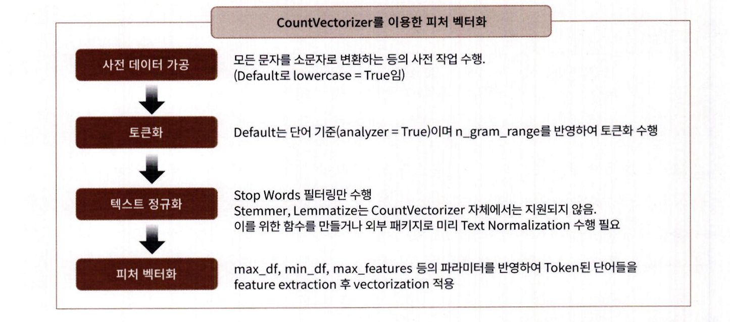
CountVectorizer 동작 순서
1. 모든 문자를 소문자 변환
2. n-gram 기반 단어 단위 토큰화 (기본: unigram)
3. 정규화 수행
4. 지정된 조건에 따라 단어 벡터화 수행

사이킷런에서 TF-IDF 벡터화는 Tfidfvectorizer 클래스를 이용합니다.

BOW 벡터화를 위한 희소 행렬

• CountVectorizer / TfidfVectorizer 변환 결과 → 텍스트 데이터를 CSR(Compressed Sparse Row) 희소 행렬 형태로 반환

희소 행렬(Sparse Matrix)

• 전체 데이터 중 0이 대부분을 차지하는 행렬
• 문서마다 단어 사용이 제한적이기 때문에 대부분의 피처 값은 0

피처 수 증가 요인

• 모든 문서의 고유 단어 → 수만~수십만 개 단어

• n-gram 설정 증가 (예: (1,2), (1,3)) → 피처 수 급증

• 벡터화된 결과는 대부분 희소 행렬

• ML 모델의 성능, 속도에 영향을 주므로 희소 행렬 특성 이해 필요

COO(Compressed Coordinate) 형식은 희소 행렬을 3개의 1차원 배열로 구성해 저장합니다.

구성 요소:
data: 0이 아닌 실제 값들
row: 각 값이 위치한 행 인덱스
col: 각 값이 위치한 열 인덱스

희소 행렬 - COO 형식

• COO(Coordinate) 형식은 0이 아닌 데이터만 따로 저장하고, 그 데이터의 행(row)과 열(column) 위치를 별도 배열에 저장하는 방식입니다.
  예를 들어 2차원 배열 [[3, 0, 1], [0, 2, 0]]이 있으면,
• 0이 아닌 값: [3, 1, 2]
• 위치: (0,0), (0,2), (1,1)
• row 배열: [0, 0, 1], column 배열: [0, 2, 1]

Python에서는 보통 SciPy의 sparse 모듈을 사용해 COO 형식의 희소 행렬로 변환합니다.

import numpy as np

dense = np.array( [ [ 3, 0, 1 ], [0, 2, 0 ] ] )

• 밀집 행렬을 scipy의 coo_matrix 클래스로 COO 형식 희소 행렬로 변환 가능
• 0이 아닌 데이터 배열, 행 위치 배열, 열 위치 배열을 각각 생성

이 세 배열을 coo_matrix()의 입력 파라미터로 전달하여 희소 행렬 생성

from scipy import sparse

# 0 이 아닌 데이터 추출
data = np.array([3,1,2])

# 행 위치와 열 위치를 각각 array로 생성 
row_pos = np.array([0,0,1])
col_pos = np.array([0,2,1])

# sparse 패키지의 coo_matrix를 이용하여 COO 형식으로 희소 행렬 생성
sparse_coo = sparse.coo_matrix((data, (row_pos,col_pos)))

sparse_coo COO 형식의 희소 행렬 객체 변수입니다. 이를 toarray() 메서드를 이용해 다시 밀집
형태의 행렬로 출력해 보겠습니다.

sparse_coo.toarray()

희소 행렬 - CSR 형식

CSR(Compressed Sparse Row) 형식은 COO 형식이 행과 열의 위치를 나타내기 위해서 반복적인
위치 데이터를 사용해야 하는 문제점을 해결한 방식입니다. 먼저 COO 변환 형식의 문제점을 알아보
겠습니다. 다음과 같은 2 차원 배열을 COO 형식으로 변환해 보겠습니다.

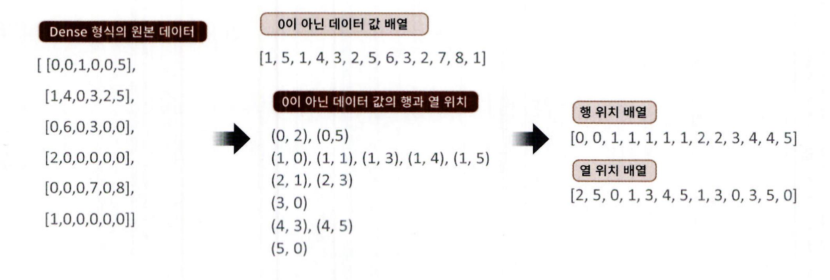
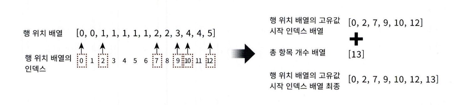
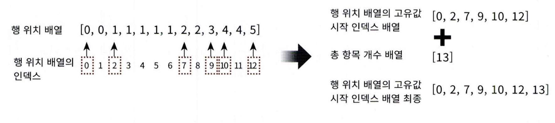
• 행 위치 배열에서 같은 값이 반복되므로, 고유값의 시작 위치만 저장하면 효율적
• 이 방식이 CSR(Compressed Sparse Row) 형식
• 원래 행 위치 배열 → [0, 0, 1, 1, 1, 1, 1, 2, 2, 3, 4, 4, 5]
  CSR 변환 후 위치 배열 → [0, 2, 7, 9, 10, 12, 13]
• 마지막 값 13은 전체 데이터 수
• CSR 형식은 메모리 절약과 연산 속도 향상에 유리함

CSR 방식의 변환은 사이파이의 csr_matrix 클래스를 이용해 쉽게 할 수 있습니다. 0 이 아닌 데이터 배
열과 열 위치 배열 , 그리고 행 위치 배열의 고유한 값의 시작 위치 배열을 csr_matrix 의 생성 파라미터
로 입력하면 됩니다.

from scipy import sparse

dense2 = np.array([[0,0,1,0,0,5],
             [1,4,0,3,2,5],
             [0,6,0,3,0,0],
             [2,0,0,0,0,0],
             [0,0,0,7,0,8],
             [1,0,0,0,0,0]])

# 0 이 아닌 데이터 추출
data2 = np.array([1, 5, 1, 4, 3, 2, 5, 6, 3, 2, 7, 8, 1])

# 행 위치와 열 위치를 각각 array로 생성 
row_pos = np.array([0, 0, 1, 1, 1, 1, 1, 2, 2, 3, 4, 4, 5])
col_pos = np.array([2, 5, 0, 1, 3, 4, 5, 1, 3, 0, 3, 5, 0])

# COO 형식으로 변환 
sparse_coo = sparse.coo_matrix((data2, (row_pos,col_pos)))

# 행 위치 배열의 고유한 값들의 시작 위치 인덱스를 배열로 생성
row_pos_ind = np.array([0, 2, 7, 9, 10, 12, 13])

# CSR 형식으로 변환 
sparse_csr = sparse.csr_matrix((data2, col_pos, row_pos_ind))

print('COO 변환된 데이터가 제대로 되었는지 다시 Dense로 출력 확인')
print(sparse_coo.toarray())
print('CSR 변환된 데이터가 제대로 되었는지 다시 Dense로 출력 확인')
print(sparse_csr.toarray())

COO 와 CSR 이 어떻게 희소 행렬의 메모리를 줄일 수 있는지 지금까지 예제를 통해서 살펴봤습니다.
실제 사용 시에는 다음과 같이 밀집 행렬을 생성 파라미터로 입력하면 COOL CSR 희소 행렬로 생성
합니다.

dense3 = np.array([[0,0,1,0,0,5],
             [1,4,0,3,2,5],
             [0,6,0,3,0,0],
             [2,0,0,0,0,0],
             [0,0,0,7,0,8],
             [1,0,0,0,0,0]])

coo = sparse.coo_matrix(dense3)
csr = sparse.csr_matrix(dense3)

여러 가지 유형의 텍스트 분석을 실제로 구현

---

텍스트 분류 실습 - 20 뉴스그룹 분류

• 사이킷런은 fetch_20newsgroups() API로 뉴스그룹 분류 예제 데이터 제공
• 텍스트 → 피처 벡터화 → 희소 행렬 형태로 변환됨

적합한 분류 알고리즘:

• 로지스틱 회귀 (Logistic Regression)
• 선형 SVM (Support Vector Machine)
• 나이브 베이즈 (Naive Bayes)

분류 과정:

• 텍스트 정규화
• 피처 벡터화 (Count, TF-IDF 방식 비교)
• 머신러닝 알고리즘 적용
• 예측 및 평가

고급 기법:

• GridSearchCV를 통한 하이퍼 파라미터 튜닝
• Pipeline으로 벡터화 + 튜닝 절차 통합 수행

텍스트 정규화

fetch_20newsgroups()는 인터넷에서 로컬 컴퓨터로 데이터를 먼저 내려받은 후에 메모리로 데이터
를 로딩합니다. 수행하려는 컴퓨터에 인터넷 연결이 정상적으로 되는지 확인한 후에 다음 예제를 수행
합니다.

from sklearn.datasets import fetch_20newsgroups

news_data = fetch_20newsgroups(subset='all',random_state=156)

fetch_20newsgroups( ) 는 사이킷런의 다른 데이터 세트 예제와 같이 파이썬 딕셔너리와 유사한
Bunch 객체를 반환합니다. 어떠한 key 값을 가지고 있는지 확인해 보겠습니다.

print(news_data.keys())

• fetch_20newsgroups() API는 load_xxx() 계열 API와 유사한 구조의 Key 값을 가짐
• 주요 key 예: data, target, target_names, filenames
  filenames: 인터넷에서 내려받은 뉴스 그룹 파일들의 로컬 저장 경로
  target: 각 문서에 대응하는 클래스 레이블(정수)
  target_names: 클래스 레이블에 대응하는 카테고리 이름 리스트

import pandas as pd

print('target 클래스의 값과 분포도 \n',pd.Series(news_data.target).value_counts().sort_index())
print('target 클래스의 이름들 \n',news_data.target_names)

Target 클래스의 값은 0 부터 19 까지 20 개로 구성돼 있으며 , 위의 출력 결과처럼 주어졌습니다 (Target
값 0: alt.atheism, Target 값 1: comp.graphics, . ) . 개별 데이터가 텍스트로 어떻게 구성돼 있는
지 데이터를 한 개만 추출해 값을 확인해 보겠습니다.

print(news_data.data[0])

• 뉴스그룹 데이터에는 제목, 작성자, 소속, 이메일 등 메타정보가 포함되어 있음
• 이 정보들은 Target 클래스와 유사한 값을 가지므로, 포함 시 예측 성능이 인위적으로 높아짐
• 따라서 텍스트 본문 내용만을 사용해 분류하는 것이 목적에 부합
• fetch_20newsgroups()의 remove 파라미터로 헤더(header), 푸터(footer) 등을 제거 가능
• subset 파라미터를 통해 학습용(train)과 테스트용(test) 데이터 세트를 분리해 다운로드 가능

from sklearn.datasets import fetch_20newsgroups

# subset='train'으로 학습용(Train) 데이터만 추출, remove=('headers', 'footers', 'quotes')로 내용만 추출
train_news= fetch_20newsgroups(subset='train', remove=('headers', 'footers', 'quotes'), random_state=156)
X_train = train_news.data
y_train = train_news.target
print(type(X_train))

# subset='test'으로 테스트(Test) 데이터만 추출, remove=('headers', 'footers', 'quotes')로 내용만 추출
test_news= fetch_20newsgroups(subset='test',remove=('headers', 'footers','quotes'),random_state=156)
X_test = test_news.data
y_test = test_news.target
print('학습 데이터 크기 {0} , 테스트 데이터 크기 {1}'.format(len(train_news.data) , len(test_news.data)))

피처 벡터화 변환과 머신러닝 모델 학습 / 예측 / 평가

• 학습 데이터: 11,314개 뉴스 문서
• 테스트 데이터: 7,532개 뉴스 문서
• CountVectorizer로 텍스트 → 피처 벡터화 진행
• 테스트 데이터는 학습에 사용된 CountVectorizer 객체의 transform()만 사용해야 함
• fit()은 피처(단어 사전)를 새로 생성하기 때문에, 학습/예측 시 피처 개수가 달라질 수 있음

from sklearn.feature_extraction.text import CountVectorizer

# Count Vectorization으로 feature extraction 변환 수행. 
cnt_vect = CountVectorizer()

cnt_vect.fit(X_train)
X_train_cnt_vect = cnt_vect.transform(X_train)

# 학습 데이터로 fit( )된 CountVectorizer를 이용하여 테스트 데이터를 feature extraction 변환 수행. 
X_test_cnt_vect = cnt_vect.transform(X_test)

print('학습 데이터 Text의 CountVectorizer Shape:',X_train_cnt_vect.shape)

학습 데이터를 CountVectorizer로 피처를 추출한 결과 11314 개의 문서에서 피처 , 즉 단어가 101631
개로 만들어졌습니다. 이렇게 피처 벡터화된 데이터에 로지스틱 회귀를 적용해 뉴스그룹에 대한 분류
를 예측해 보겠습니다.

from sklearn.linear_model import LogisticRegression
from sklearn.metrics import accuracy_score
import warnings
warnings.filterwarnings('ignore')

# LogisticRegression을 이용하여 학습/예측/평가 수행. 
lr_clf = LogisticRegression(solver='liblinear')
lr_clf.fit(X_train_cnt_vect , y_train)
pred = lr_clf.predict(X_test_cnt_vect)
print('CountVectorized Logistic Regression 의 예측 정확도는 {0:.3f}'.format(accuracy_score(y_test,pred)))

Count 기반으로 피처 벡터화가 적용된 데이터 세트에 대한 로지스틱 회귀의 예측 정확도는 약 0.616
입니다. 이번에는 Count 기반에서 TF-IDF 기반으로 벡터화를 변경해 예측 모델을 수행하겠습니다.

from sklearn.feature_extraction.text import TfidfVectorizer

# TF-IDF Vectorization 적용하여 학습 데이터셋과 테스트 데이터 셋 변환. 
tfidf_vect = TfidfVectorizer()
tfidf_vect.fit(X_train)
X_train_tfidf_vect = tfidf_vect.transform(X_train)
X_test_tfidf_vect = tfidf_vect.transform(X_test)

# LogisticRegression을 이용하여 학습/예측/평가 수행. 
lr_clf = LogisticRegression(solver='liblinear')
lr_clf.fit(X_train_tfidf_vect , y_train)
pred = lr_clf.predict(X_test_tfidf_vect)
print('TF-IDF Logistic Regression 의 예측 정확도는 {0:.3f}'.format(accuracy_score(y_test ,pred)))

• TF-IDF는 단순 Count보다 예측 정확도가 더 높음
• 많은 문서, 긴 텍스트일수록 TF-IDF가 효과적임
• 텍스트 분석 성능 향상 요인:
  적절한 머신러닝 알고리즘 선택
  효과적인 피처 전처리

# stop words 필터링을 추가하고 ngram을 기본(1,1)에서 (1,2)로 변경하여 Feature Vectorization 적용.
tfidf_vect = TfidfVectorizer(stop_words='english', ngram_range=(1,2), max_df=300 )
tfidf_vect.fit(X_train)
X_train_tfidf_vect = tfidf_vect.transform(X_train)
X_test_tfidf_vect = tfidf_vect.transform(X_test)

lr_clf = LogisticRegression(solver='liblinear')
lr_clf.fit(X_train_tfidf_vect , y_train)
pred = lr_clf.predict(X_test_tfidf_vect)
print('TF-IDF Vectorized Logistic Regression 의 예측 정확도는 {0:.3f}'.format(accuracy_score(y_test ,pred)))

GridSearchCV 를 이용해 로지스틱 회귀의 하이퍼 파라미터 최적화를 수행해 보겠습니다. 로
지스틱 회귀의 C 파라미터만 변경하면서 최적의 C 값을 찾은 뒤 이 C 값으로 학습된 모델에서 테스트 데
이터로 예측해 성능을 평가하겠습니다.

from sklearn.model_selection import GridSearchCV

# 최적 C 값 도출 튜닝 수행. CV는 3 Fold셋으로 설정. 
params = { 'C':[0.01, 0.1, 1, 5, 10]}
grid_cv_lr = GridSearchCV(lr_clf ,param_grid=params , cv=3 , scoring='accuracy' , verbose=1 )
grid_cv_lr.fit(X_train_tfidf_vect , y_train)
print('Logistic Regression best C parameter :',grid_cv_lr.best_params_ )

# 최적 C 값으로 학습된 grid_cv로 예측 수행하고 정확도 평가. 
pred = grid_cv_lr.predict(X_test_tfidf_vect)
print('TF-IDF Vectorized Logistic Regression 의 예측 정확도는 {0:.3f}'.format(accuracy_score(y_test ,pred)))

로지스틱 회귀의 C 가 10일 때 GridSearchCV의 교차 검증 테스트 세트에서 가장 좋은 예측 성능을 나
타냈으며 , 이를 테스트 데이터 세트에 적용해 약 0.704 로 이전보다 약간 향상된 성능 수치가 됐습니다.

사이킷런 파이프라인 (Pipeline) 사용 및 GridSearchCV와의 결합

사이킷런의 Pipeline 클래스는

• 피처 벡터화 + ML 학습/예측을 한 줄처럼 처리
• 전처리와 모델링을 스트림(stream) 방식으로 연결

장점:

• 코드 직관적
• 대용량 데이터 처리 효율적
• 벡터화 결과를 별도 저장 없이 바로 모델에 전달
• 모든 전처리 (예: 스케일링, PCA) 와 Estimator 결합 가능

Pipeline([('vectorizer', CountVectorizer()), ('clf', LogisticRegression())])

0 텍스트 분류, 수치형 데이터 모델링 등 다양한 작업에 활용 가능

from sklearn.pipeline import Pipeline

# TfidfVectorizer 객체를 tfidf_vect 객체명으로, LogisticRegression객체를 lr_clf 객체명으로 생성하는 Pipeline생성
pipeline = Pipeline([
    ('tfidf_vect', TfidfVectorizer(stop_words='english', ngram_range=(1,2), max_df=300)),
    ('lr_clf', LogisticRegression(solver='liblinear', C=10))
])

# 별도의 TfidfVectorizer객체의 fit_transform( )과 LogisticRegression의 fit(), predict( )가 필요 없음. 
# pipeline의 fit( ) 과 predict( ) 만으로 한꺼번에 Feature Vectorization과 ML 학습/예측이 가능. 
pipeline.fit(X_train, y_train)
pred = pipeline.predict(X_test)
print('Pipeline을 통한 Logistic Regression 의 예측 정확도는 {0:.3f}'.format(accuracy_score(y_test ,pred)))

• 사이킷런의 GridSearchCV는
  Pipeline 객체도 입력 가능하여→ 피처 벡터화 + 모델 하이퍼파라미터를 동시에 최적화할 수 있음.

• param_grid의 key 값은 "객체명__파라미터명" 형식 사용

예: tfidf_vect__ngram_range

너무 많은 파라미터 조합은 시간이 많이 소요됨
→ (예: 27 조합 × 3 CV = 81회 실행 → 약 24분)

• 벡터화와 모델의 파라미터를 함께 자동 탐색 가능
• 전체 모델 최적화 프로세스를 통합하여 효율적

from sklearn.pipeline import Pipeline

pipeline = Pipeline([
    ('tfidf_vect', TfidfVectorizer(stop_words='english')),
    ('lr_clf', LogisticRegression(solver='liblinear'))
])

# Pipeline에 기술된 각각의 객체 변수에 언더바(_)2개를 연달아 붙여 GridSearchCV에 사용될 
# 파라미터/하이퍼 파라미터 이름과 값을 설정. . 
params = { 'tfidf_vect__ngram_range': [(1,1), (1,2), (1,3)],
           'tfidf_vect__max_df': [100, 300, 700],
           'lr_clf__C': [1, 5, 10]
}

# GridSearchCV의 생성자에 Estimator가 아닌 Pipeline 객체 입력
grid_cv_pipe = GridSearchCV(pipeline, param_grid=params, cv=3 , scoring='accuracy',verbose=1)
grid_cv_pipe.fit(X_train , y_train)
print(grid_cv_pipe.best_params_ , grid_cv_pipe.best_score_)

pred = grid_cv_pipe.predict(X_test)
print('Pipeline을 통한 Logistic Regression 의 예측 정확도는 {0:.3f}'.format(accuracy_score(y_test ,pred)))

5. 감성 분석

• 감성 분석(Sentiment Analysis)은
  문서 속 감정, 의견, 기분, 태도 등 주관적 정보를 파악하는 기법입니다.
• 활용 분야: 소셜 미디어, 여론조사, 온라인 리뷰, 고객 피드백 등
  분석 방법:
• 문맥과 주관적 단어를 기반으로
• 긍정/부정 감성 점수를 계산
• 두 점수의 합산으로 전체 감성을 판단

분류 방식:

• 지도학습(Supervised learning)
  감성 레이블이 있는 학습 데이터를 사용
  이를 기반으로 새로운 텍스트의 감성을 예측
  일반적인 텍스트 분류 방식과 유사

• 비지도학습(Unsupervised learning)
  Lexicon(감성 어휘 사전)을 활용
  단어와 문맥의 감성 정보를 바탕으로
  문서가 긍정적인지 부정적인지 판단

지도 학습은 데이터 기반 학습 → 예측
비지도 학습은 사전 기반 규칙 → 판단

지도학습 기반 감성 분석 실습 - IMDB 영화평

• 다운로드한 압축 파일을 해제하고 labeledTrainData.tsv 파일을 사용함
• 해당 파일을 노트북 디렉터리로 이동
• labeledTrainData.tsv는 탭(\t)으로 구분된 TSV 파일
• Pandas의 read_csv()로 불러올 수 있음
• 이때 sep="\t"를 명시해야 함

import pandas as pd

review_df = pd.read_csv('/content/sample_data/labeledTrainData.tsv', header=0, sep="\t", quoting=3)
review_df.head(3)

피처

• id :
• sentiment : 영화평의 Sentiment결과 값 (Target Label) 1은 긍정적 평가 , 0 은 부정적 평가
• review : 영화평의 텍스트

텍스트가 어떻게 구성돼 있는지 확인 (html형식)

print(review_df['review'][0])

• HTML 태그
  제거: 불필요하므로 공백으로 바꿈
• Pandas의 str.replace() 사용
  숫자 및 특수문자 제거: 감성 분석에 의미 없으므로 제거
• 정규표현식 + re.sub() 사용
• Pandas에서는 lambda 적용

import re

# <br> html 태그는 replace 함수로 공백으로 변환
review_df['review'] = review_df['review'].str.replace('<br />',' ')

# 파이썬의 정규 표현식 모듈인 re를 이용하여 영어 문자열이 아닌 문자는 모두 공백으로 변환 
review_df['review'] = review_df['review'].apply( lambda x : re.sub("[^a-zA-Z]", " ", x) )

• sentiment 칼럼만 따로 추출 → 타깃 데이터셋 (레이블) 생성
• 원본 데이터에서 id, sentiment 칼럼 제거 → 피처 데이터셋 생성
• train_test_split() 함수 사용해 학습용 / 테스트용 데이터로 분리

from sklearn.model_selection import train_test_split

class_df = review_df['sentiment']
feature_df = review_df.drop(['id','sentiment'], axis=1, inplace=False)

X_train, X_test, y_train, y_test= train_test_split(feature_df, class_df, test_size=0.3, random_state=156)

X_train.shape, X_test.shape

• 학습 데이터: 17,500개 리뷰, 테스트 데이터: 7,500개 리뷰

• CountVectorizer : 벡터화

• LogisticRegression : 분류 적용

• Pipeline 사용해 벡터화 + 분류를 한꺼번에 수행

• 평가 지표:
  정확도 (Accuracy)
  ROC-AUC (이진 분류이므로 사용)

from sklearn.feature_extraction.text import CountVectorizer, TfidfVectorizer
from sklearn.pipeline import Pipeline
from sklearn.linear_model import LogisticRegression
from sklearn.metrics import accuracy_score, roc_auc_score

# 스톱 워드는 English, filtering, ngram은 (1,2)로 설정해 CountVectorization수행. 
# LogisticRegression의 C는 10으로 설정. 
pipeline = Pipeline([
    ('cnt_vect', CountVectorizer(stop_words='english', ngram_range=(1,2) )),
    ('lr_clf', LogisticRegression(solver='liblinear', C=10))])

# Pipeline 객체를 이용하여 fit(), predict()로 학습/예측 수행. predict_proba()는 roc_auc때문에 수행.  
pipeline.fit(X_train['review'], y_train)
pred = pipeline.predict(X_test['review'])
pred_probs = pipeline.predict_proba(X_test['review'])[:,1]

print('예측 정확도는 {0:.4f}, ROC-AUC는 {1:.4f}'.format(accuracy_score(y_test ,pred),
                                         roc_auc_score(y_test, pred_probs)))

• 이번에는 이전과 동일한 방식으로 TF-IDF 벡터화를 사용하여 다시 예측 성능을 측정합니다.

TfidfVectorizer 적용

# 스톱 워드는 english, filtering, ngram은 (1,2)로 설정해 TF-IDF 벡터화 수행. 
# LogisticRegression의 C는 10으로 설정. 
pipeline = Pipeline([
    ('tfidf_vect', TfidfVectorizer(stop_words='english', ngram_range=(1,2) )),
    ('lr_clf', LogisticRegression(solver='liblinear', C=10))])

pipeline.fit(X_train['review'], y_train)
pred = pipeline.predict(X_test['review'])
pred_probs = pipeline.predict_proba(X_test['review'])[:,1]

print('예측 정확도는 {0:.4f}, ROC-AUC는 {1:.4f}'.format(accuracy_score(y_test ,pred),
                                         roc_auc_score(y_test, pred_probs)))

TF-IDF 기반 피처 벡터화의 예측 성능이 조금 더 나아짐

비지도학습 기반 감성 분석 소개

• 비지도 감성 분석은 Lexicon(감성 어휘 사전) 기반 방식입니다. 라벨이 없는 데이터에도 사용할 수 있어 유용합니다.

• Lexicon(감성 사전): 긍정/부정 감성의 정도를 수치화한 Polarity Score 보유

• 문맥, 주변 단어, 품사 등을 고려해 감성 점수 부여

• 구현: NLTK의 Lexicon 모듈

• WordNet: 영어 단어의 시맨틱(문맥 의미) 정보 제공

• 단어는 문맥에 따라 의미 달라지므로, 이를 Synset(동의어 집합)으로 표현함

• NLTK의 감성 사전은 감성 분석의 기초 자료로는 훌륭하지만, 예측 성능이 낮다는 한계가 있음

• 따라서 실제 업무에서는 NLTK 외의 다른 감성 사전을 사용하는 경우가 많습니다.

대표적인 감성 사전

SentiWordNet:

• WordNet의 Synset 개념을 기반으로 긍정 점수, 부정 점수, 객관성 점수를 각 단어에 부여
• 문장의 감성은 단어들의 점수를 합산하여 결정

VADER:

• 소셜 미디어 텍스트에 특화된 감성 분석 패키지로, 빠른 속도와 우수한 성능 덕분에 대용량 텍스트 분석에 자주 사용

Pattern:

• 높은 예측 성능으로 주목받았지만, 현재는 Python 2.x에서만 작동하며

• SentiWordNet과 VADER를 이용한 감성 분석 결과를 지도 학습 기반 분류 모델과 비교함
• SentiWordNet은 예측 정확도가 낮아 실무에서 자주 사용되지는 않지만, 감성 사전이 시맨틱 기반으로 어떻게 구성되는지 이해하는 데 유용함
• 실용적인 감성 분석은 VADER만 참고해도 충분하며, WordNet 기반 시맨틱 방식에 관심이 없다면 VADER 부분부터 학습해도 무방함

SentiWordNet을 이용한 감성 분석

• SentiWordNet은 WordNet 기반의 Synset을 사용하므로, Synset 개념을 먼저 이해해야 함.
• 사용 전, NLTK 설치 및 WordNet 서브 패키지와 데이터셋 다운로드 필요.
• nltk.download('all') 실행 시 많은 데이터가 포함되므로 다운로드에 시간이 꽤 걸림.

import nltk
nltk.download('all')

• NLTK 데이터셋을 모두 다운로드한 뒤, WordNet 모듈을 import 하고, present 단어에 대한 Synset을 추출함.
• wordnet.synsets('present')를 사용하면 WordNet에 등록된 모든 Synset 객체 목록이 반환됨.

from nltk.corpus import wordnet as wn

term = 'present'

# 'present'라는 단어로 wordnet의 synsets 생성. 
synsets = wn.synsets(term)
print('synsets() 반환 type :', type(synsets))
print('synsets() 반환 값 갯수:', len(synsets))
print('synsets() 반환 값 :', synsets)

• synsets() 호출 결과: 여러 개의 synset 객체를 가지는 리스트 반환됨

• present: 단어 의미

• n: POS 태그 (명사)

• 01: 동일 품사 내 의미 인덱스

• synset 객체는 다음 속성 포함:
  POS (Part of Speech)
  정의 (Definition)
  부명제 (Lemma)

for synset in synsets :
    print('##### Synset name : ', synset.name(),'#####')
    print('POS :',synset.lexname())
    print('Definition:',synset.definition())
    print('Lemmas:',synset.lemma_names())

Synset('present.n.01')

• 명사 noun.time
• 의미: ‘시간적인 의미로 현재’

Synset('present.n.02')

• 명사 noun.possession
• 의미: ‘선물’

Synset('show.v.01')

• 동사 verb.perception

• 의미: ‘관객에게 전시물 등을 보여주다’

• Synset은 하나의 단어가 가지는 다양한 의미(시맨틱 정보)를 개별 클래스로 표현함

WordNet은 단어 간 유사도를 나타낼 수 있음

• path_similarity() 메서드 사용
• 예시 단어: 'tree', 'lion', 'tiger', 'cat', 'dog'

# synset 객체를 단어별로 생성합니다. 
tree = wn.synset('tree.n.01')
lion = wn.synset('lion.n.01')
tiger = wn.synset('tiger.n.02')
cat = wn.synset('cat.n.01')
dog = wn.synset('dog.n.01')

entities = [tree , lion , tiger , cat , dog]
similarities = []
entity_names = [ entity.name().split('.')[0] for entity in entities]

# 단어별 synset 들을 iteration 하면서 다른 단어들의 synset과 유사도를 측정합니다. 
for entity in entities:
    similarity = [ round(entity.path_similarity(compared_entity), 2)  for compared_entity in entities ]
    similarities.append(similarity)
    
# 개별 단어별 synset과 다른 단어의 synset과의 유사도를 DataFrame형태로 저장합니다.  
similarity_df = pd.DataFrame(similarities , columns=entity_names,index=entity_names)
similarity_df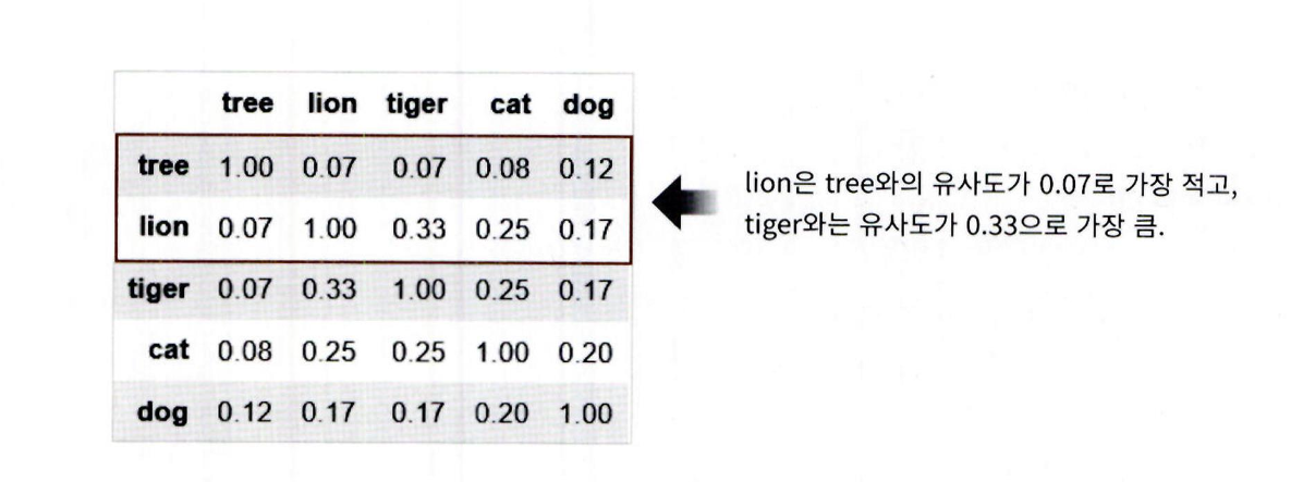

• SentiWordNet은 WordNet의 Synset과 유사한
• Senti_Synset 클래스를 가짐

senti_synsets() 함수는

• WordNet의 synsets()처럼 동작
• Senti_Synset 객체들을 리스트 형태로 반환함

import nltk
from nltk.corpus import sentiwordnet as swn

senti_synsets = list(swn.senti_synsets('slow'))
print('senti_synsets() 반환 type :', type(senti_synsets))
print('senti_synsets() 반환 값 갯수:', len(senti_synsets))
print('senti_synsets() 반환 값 :', senti_synsets)

• SentiSynset 객체는 단어의 감성을 나타내는
  긍정 감성 지수, 부정 감성 지수, 그리고
  객관성 지수(= 1 − 감성 지수 합)을 가짐

father → 감성 지수: 거의 0 → 객관성 지수: 1
fabulous → 긍정 감성 지수 높음 → 객관성 지수 낮음

import nltk
from nltk.corpus import sentiwordnet as swn

father = swn.senti_synset('father.n.01')
print('father 긍정감성 지수: ', father.pos_score())
print('father 부정감성 지수: ', father.neg_score())
print('father 객관성 지수: ', father.obj_score())
print('\n')
fabulous = swn.senti_synset('fabulous.a.01')
print('fabulous 긍정감성 지수: ',fabulous .pos_score())
print('fabulous 부정감성 지수: ',fabulous .neg_score())

**father: 감성 단어가 아님** 
- 긍정 감성 지수 = 0
- 부정 감성 지수 = 0
- 객관성 지수 = 1.0 (매우 객관적인 단어)

**fabulous: 감성 단어 **
- 긍정 감성 지수 = 0.875
- 부정 감성 지수 = 0.125
- 객관성 지수 < 1.0 (감성 포함됨)

감성 사전은 단어가 감성적인지 객관적인지 수치로 구분


## SentiWordNet을 이용한 영화 감상평 감성 분석 

SentiWordNet을 활용한 IMDB 영화 리뷰 감성 분석의 전체 순서는 다음과 같다


1. 문서(Document)를 문장(Sentence) 단위로 분해

2. 다시 문장을 단어(Word) 단위로 토큰화하고 품사 태깅

3. 품사 태깅된 단어 기반으로 Synset 객체와 Senti_Synset 객체를 생성

4. Senti_Synset 객체에서 긍정 감성 / 부정 감성 지수를 구하고 이를 모두 합산해 특정 임계치 값 이상일 때 긍정 감성으로, 그렇지 않을 때는 부정 감성으로 결정

SentiWordNet을 이용하기 위해서 WordNet을 이용해 문서를 다시 단어로 토큰화한 뒤, 어근 추출(Lemmatization)과 품사 태깅(PoS Tagging)을 적용해야 합니다.
먼저, 품사 태깅을 수행하는 내부 함수를 생성하겠습니다.


 

from nltk.corpus import wordnet as wn

간단한 NTLK PennTreebank Tag를 기반으로 WordNet기반의 품사 Tag로 변환

def penn_to_wn(tag):
if tag.startswith('J'):
return wn.ADJ
elif tag.startswith('N'):
return wn.NOUN
elif tag.startswith('R'):
return wn.ADV
elif tag.startswith('V'):
return wn.VERB
return

----

- 문서를 문장 - 단어 토큰 - 품사 태깅 후에 SentiSynset 클래스를 생성하고, Polarity Score를 합산하는 함수를 생성
- 각 단어의 긍정 감성 지수와 부정 감성 지수를 모두 합한 총 감성 지수가 0 이상일 경우 긍정 감성, 그렇지 않을 경우 부정 감성으로 예측

from nltk.stem import WordNetLemmatizer
from nltk.corpus import sentiwordnet as swn
from nltk import sent_tokenize, word_tokenize, pos_tag

def swn_polarity(text):

# 감성 지수 초기화 
sentiment = 0.0
tokens_count = 0

lemmatizer = WordNetLemmatizer()
raw_sentences = sent_tokenize(text)
# 분해된 문장별로 단어 토큰 -> 품사 태깅 후에 SentiSynset 생성 -> 감성 지수 합산 
for raw_sentence in raw_sentences:
    # NTLK 기반의 품사 태깅 문장 추출  
    tagged_sentence = pos_tag(word_tokenize(raw_sentence))
    for word , tag in tagged_sentence:
        
        # WordNet 기반 품사 태깅과 어근 추출
        wn_tag = penn_to_wn(tag)
        if wn_tag not in (wn.NOUN , wn.ADJ, wn.ADV):
            continue                   
        lemma = lemmatizer.lemmatize(word, pos=wn_tag)
        if not lemma:
            continue
        # 어근을 추출한 단어와 WordNet 기반 품사 태깅을 입력해 Synset 객체를 생성. 
        synsets = wn.synsets(lemma , pos=wn_tag)
        if not synsets:
            continue
        # sentiwordnet의 감성 단어 분석으로 감성 synset 추출
        # 모든 단어에 대해 긍정 감성 지수는 +로 부정 감성 지수는 -로 합산해 감성 지수 계산. 
        synset = synsets[0]
        swn_synset = swn.senti_synset(synset.name())
        sentiment += (swn_synset.pos_score() - swn_synset.neg_score())           
        tokens_count += 1

if not tokens_count:
    return 0

# 총 score가 0 이상일 경우 긍정(Positive) 1, 그렇지 않을 경우 부정(Negative) 0 반환
if sentiment >= 0 :
    return 1

return 0

- swn_polarity(text) 함수를 IMDB 감상평 데이터셋의 각 문서에 적용해 감성(긍정/부정)을 예측함 
- 이때 pandas의 apply(lambda ...) 문법을 사용하여 review_df의 각 행에 함수 적용함 
- 예측 결과는 새로운 컬럼 'preds'에 저장됨

이후 sentiment 컬럼(실제 정답 레이블)과 비교하여 이를 평가: 
- 정확도 (Accuracy)
- 정밀도 (Precision)
- 재현율 (Recall)

review_df['preds'] = review_df['review'].apply( lambda x : swn_polarity(x) )
y_target = review_df['sentiment'].values
preds = review_df['preds'].values

SentiWordNet의 감성 분석 예측 성능 

from sklearn.metrics import accuracy_score, confusion_matrix, precision_score
from sklearn.metrics import recall_score, f1_score, roc_auc_score
import numpy as np

print(confusion_matrix( y_target, preds))
print("정확도:", np.round(accuracy_score(y_target , preds), 4))
print("정밀도:", np.round(precision_score(y_target , preds),4))
print("재현율:", np.round(recall_score(y_target, preds), 4))

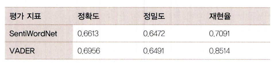
SentiWordNet 기반 감성 분석의 결과:
- 정확도: 약 66.13%
- 재현율: 약 70.91%
- 전체적으로 성능이 만족스럽지는 않음
- SentiWordNet은 WordNet을 기반으로 하지만, 성능 개선에는 한계가 있음

## VADER를 이용한 감성 분석 
- VADER는 소셜 미디어 텍스트의 감성 분석을 위해 만들어진 룰 기반의 Lexicon이음.
- SentimentIntensityAnalyzer 클래스를 이용해 감성 점수를 쉽게 계산할 수 있음.
- NLTK 서브모듈로 제공되며, 별도 설치 없이 사용할 수 있음.
- 또는 pip install vaderSentiment로 설치한 뒤 사용할 수도 있음.
- 문장에 대해 긍정, 부정, 중립, 종합 점수를 반환함.
- 버전에 따라 출력 결과는 다를 수 있음.

from nltk.sentiment.vader import SentimentIntensityAnalyzer

senti_analyzer = SentimentIntensityAnalyzer()
senti_scores = senti_analyzer.polarity_scores(review_df['review'][0])
print(senti_scores)

- VADER를 이용하면 매우 쉽게 감성 분석을 수행할 수 있음.
- 먼저 SentimentIntensityAnalyzer 객체를 생성한 뒤, 각 문서에 대해 
- polarity_scores() 메서드를 호출하여 감성 점수를 구함.
- polarity_scores()는 네 가지 점수인 'neg', 'neu', 'pos', 'compound'를 포함한 딕셔너리를 반환함.
- 'compound' 점수는 -1에서 1 사이의 값으로 전체적인 감성의 강도를 나타냄.
- 보통 compound 값이 0.1 이상이면 긍정, 이하면 부정으로 간주함.
- 상황에 따라 이 임계값은 조정될 수 있음.
- vader_polarity() 함수를 정의해 감성 분석을 자동화하고, apply(lambda)를 통해 각 문서에 적용해 결과를 저장함.
- 해당 결과를 이용해 VADER의 예측 성능을 측정함.

def vader_polarity(review,threshold=0.1):
analyzer = SentimentIntensityAnalyzer()
scores = analyzer.polarity_scores(review)

# compound 값에 기반하여 threshold 입력값보다 크면 1, 그렇지 않으면 0을 반환 
agg_score = scores['compound']
final_sentiment = 1 if agg_score >= threshold else 0
return final_sentiment

apply lambda 식을 이용하여 레코드별로 vader_polarity( )를 수행하고 결과를 'vader_preds'에 저장

review_df['vader_preds'] = review_df['review'].apply( lambda x : vader_polarity(x, 0.1) )
y_target = review_df['sentiment'].values
vader_preds = review_df['vader_preds'].values

print(confusion_matrix( y_target, vader_preds))
print("정확도:", np.round(accuracy_score(y_target , vader_preds),4))
print("정밀도:", np.round(precision_score(y_target , vader_preds),4))
print("재현율:", np.round(recall_score(y_target, vader_preds),4))

정확도가 SentiWordNet보다 향상됐고, 특히 재현율은 약 85.14%로 매우 크게 향상됐음.
이 외에도 뛰어난 감성 사전으로 pattern 패키지가 있음.

![](https://velog.velcdn.com/images/nunnalin/post/2ef25d8f-2cee-4e4a-ae39-8db3b5fd5f45/image.png)

- 감성 사전을 이용한 감성 분석 예측 성능은 지도 학습 분류 기반의 예측 성능에 비해 아직은 낮은 수준임.
- 그러나 결정 클래스 값이 없는 상황을 고려한다면 예측 성능에 일정 수준 만족할 수 있을 것임.

### 토픽 모델링 (Topic Modeling) - 20뉴스그룹 
- 토픽 모델링이란 문서 집합에서 숨겨진 주제를 자동으로 찾아내는 작업임.
- 사람이 직접 모든 문서를 읽고 핵심 주제를 파악하는 것은 비효율적이므로, 머신러닝 기반 방법을 통해 핵심 단어를 추출해 효율적으로 표현함.
- 머신러닝 기반 토픽 모델링 기법에는 LSA와 LDA가 있으나, 여기서는 LDA(Latent Dirichlet Allocation)만 사용함.
- 이 LDA는 차원 축소 기법인 LDA(Linear Discriminant Analysis)와는 다른 알고리즘이므로 주의가 필요함.
- 실습은 앞서 사용한 20 Newsgroups 데이터셋을 활용하며, 이 데이터는 20가지 주제를 가진 뉴스 그룹으로 구성됨

**총 8개의 주제 — 모터사이클, 야구, 그래픽스, 윈도우, 중동, 기독교, 전자공학, 의학 — 을 추출하여, 이들 텍스트에 대해 LDA(Latent Dirichlet Allocation) 기반 토픽 모델링을 적용함.**
- LDA는 사이킷런에서 LatentDirichletAllocation 클래스를 통해 제공되며, 초기에는 지원되지 않았으나 gensim의 인기에 따라 추가된 기능임.
**모델링 절차는 다음과 같음:**
- fetch_20newsgroups() API에서 categories 파라미터를 사용해 필요한 주제만 필터링함.
- 텍스트는 Count 기반 벡터화로 변환함 (LDA는 TF-IDF가 아닌 Count 기반만 사용함).

**벡터화는 다음 설정을 따름:**

from sklearn.datasets import fetch_20newsgroups
from sklearn.feature_extraction.text import CountVectorizer
from sklearn.decomposition import LatentDirichletAllocation

모 터 사 이 클 , 야 구 , 그 래 픽 스 , 윈 도 우 즈 , 중 동 , 기 독 교 , 전 자 공 학 , 의 학 8 개 주 제 를 추 출 .

cats = ['rec.motorcycles'
, 'rec.sport.baseball', 'comp.graphics', 'comp.windows.x',
'talk.politics.mideast', 'soc.religion.christian', 'sci.electronics', 'sci.med']

위 에 서 c a t s 변 수 로 기 재 된 카 테 고 리 만 추 출 . f e a t c h _ 2 0 n e w s g r o u p s ( ) 의 c a t e g o r i e s 에 c a t s 입 력

news_df= fetch_20newsgroups(subset='all', remove=('headers', 'footers', 'quotes'),
categories=cats, random_state=0)

L D A 는 C o u n t 기 반 의 벡 터 화 만 적 용 합 니 다 .

count_vect = CountVectorizer(max_df=0.95, max_features=1000, min_df=2, stop_words='english',
ngram_range=(1, 2))
feat_vect = count_vect.fit_transform(news_df.data)
print( 'CountVectorizer Shape:', feat_vect.shape)

- CountVectorizer로 생성한 feat_vect는 총 7,862개의 문서와 1,000개의 피처로 구성된 행렬 데이터를 나타냄.
- 이 피처 벡터화된 데이터를 기반으로 LDA 토픽 모델링을 수행함.
- 토픽 수는 뉴스 그룹에서 추출한 주제 수와 동일하게 8개로 설정함.
- LatentDirichletAllocation 클래스의 n_components 파라미터를 통해 토픽 수를 설정하며, random_state는 실행 결과의 일관성을 위해 설정함.

lda = LatentDirichletAllocation(n_components=8, random_state=0)
lda.fit(feat_vect)

- LatentDirichletAllocation.fit(데이터셋)을 수행하면 LDA 모델 객체는 components_라는 속성을 가지게 됨.
- 이 components_ 속성은 **각 토픽마다 단어(feature)**가 얼마나 많이 해당 토픽에 할당되었는지를 나타내는 수치 행렬임.
- 형식: components_는 (n_topics, n_features) 형태의 2차원 배열
각 행(row)은 하나의 토픽
각 열(column)은 하나의 단어 피처
- 값이 클수록 해당 단어가 그 토픽의 **핵심 단어(중요 단어)**임을 의미함

print(lda.components.shape)
lda.components

components_ 값만으로는 각 토픽별 중심 단어를 사람이 이해하기 어렵기 때문에, display_topics() 함수를 만들어야 함.

def displaytopics(model, feature_names, no_top_words):
for topic_index, topic in enumerate(model.components):
print('Topic #', topic_index)
topic_word_indexes = topic.argsort()[::-1]
top_indexes=topic_word_indexes[:no_top_words]

    feature_concat = ' '.join([feature_names [i] for i in top_indexes])
    print(feature_concat)

feature_names = count_vect.get_feature_names_out()
display_topics(lda, feature_names, 15)

총 8개의 주제 중 일부는 잘 매핑되었으나, 일부는 주제가 불명확함.

- 의학, 중동, 그래픽스, 기독교, 윈도우즈 관련 토픽은 명확하게 추출됨.
- 반면 모터사이클, 야구 관련 주제는 추출되지 않았으며, Topic #1, #3, #5는 일반 단어 위주로 애매한 주제어가 포함됨.