DeepSeekMath: Pushing the Limits of Mathematical Reasoning in Open Language Models (24.02)

onpo·2026년 9월 16일

Paper Notes

목록 보기

2/6

DeepSeekMath: GRPO 이해하기

DeepSeekMath는 수학적 reasoning에 특화된 7B 규모의 언어 모델이다.

논문에서는 대규모 수학 데이터 구축과 instruction tuning뿐 아니라, PPO를 변형한 강화학습 알고리즘인 GRPO(Group Relative Policy Optimization)를 제안한다.

GRPO의 핵심은 다음과 같다.

PPO에서 advantage estimation을 위해 사용하던 Value Model을 제거하고, 같은 question에 대해 생성된 여러 response의 상대적인 reward를 이용해 advantage를 계산한다.

이 글에서는 DeepSeekMath의 전체 학습 과정은 간단히 살펴보고, 논문의 핵심인 PPO에서 GRPO로 이어지는 흐름을 중심으로 정리한다.

1. DeepSeekMath는 어떤 모델인가?

DeepSeekMath는 DeepSeek-Coder-Base-v1.5 7B를 기반으로 수학 데이터에 continual pre-training과 instruction tuning을 적용한 모델이다.

전체 학습 과정은 다음과 같다.

DeepSeek-Coder-Base 7B
        ↓
Math-centered Pre-training
        ↓
DeepSeekMath-Base
        ↓
Supervised Fine-Tuning
        ↓
DeepSeekMath-Instruct
        ↓
GRPO
        ↓
DeepSeekMath-RL

Pre-training 단계에서는 Common Crawl에서 구축한 대규모 수학 데이터를 활용하고, 이후 SFT를 통해 Chain-of-Thought, Program-of-Thought, Tool-Integrated Reasoning과 같은 다양한 풀이 형식을 학습한다.

즉 GRPO는 처음부터 수학을 학습시키는 방법이 아니라, 이미 pre-training과 SFT를 거쳐 reasoning 능력을 갖춘 DeepSeekMath-Instruct에 추가적으로 RL을 적용하는 단계이다.

이후부터는 GRPO에 집중한다.

2. PPO부터 이해하기

GRPO는 PPO의 변형이므로 먼저 PPO가 무엇을 최적화하는지 볼 필요가 있다.

PPO에서는 question dataset에서 질문을 sampling하고, old policy를 사용해 response를 생성한다.

q \sim P(Q)

o \sim \pi_{\theta_{\mathrm{old}}}(O \mid q)

그리고 다음 surrogate objective를 최대화한다.

J_{\mathrm{PPO}}(\theta) = \mathbb{E}_{q \sim P(Q),\,o \sim \pi_{\theta_{\mathrm{old}}}(O\mid q)} \left[ \frac{1}{|o|} \sum_{t=1}^{|o|} \min \left( \rho_t A_t, \operatorname{clip} \left( \rho_t, 1-\epsilon, 1+\epsilon \right) A_t \right) \right]

여기서 policy ratio는 다음과 같다.

\rho_t = \frac{ \pi_\theta(o_t\mid q,o_{<t}) }{ \pi_{\theta_{\mathrm{old}}}(o_t\mid q,o_{<t}) }

즉 old policy와 비교해 current policy가 해당 token을 생성할 확률을 얼마나 변화시켰는지 나타낸다.

2.1 PPO에서 clipping을 사용하는 이유

PPO는 current policy가 old policy에서 지나치게 크게 바뀌는 것을 제한한다.

이를 위해 policy ratio를 다음 범위로 clipping한다.

1-\epsilon \le \rho_t \le 1+\epsilon

그리고

\min \left( \rho_t A_t, \operatorname{clip}(\rho_t,1-\epsilon,1+\epsilon)A_t \right)

처럼 unclipped objective와 clipped objective 중 더 보수적인 값을 사용한다.

즉 PPO의 핵심은 advantage가 높은 action을 강화하되, 한 번의 update에서 policy가 지나치게 크게 변화하지 않도록 제한하는 것이다.

3. PPO에서 Advantage는 어떻게 계산할까?

PPO에서 중요한 값이 Advantage이다.

Advantage는 현재 action이 baseline과 비교해 얼마나 유리했는지를 나타낸다.

PPO에서는 일반적으로 reward와 learned value function을 이용해 GAE(Generalized Advantage Estimation)로 Advantage를 추정한다.

Reward
   +
Value Model
   ↓
GAE
   ↓
Advantage

즉 policy model 외에도

현재 state에서 앞으로 받을 return을 추정하는 Value Model

이 필요하다.

문제는 LLM의 크기가 커질수록 Value Model 역시 상당히 큰 별도 모델이 될 수 있다는 것이다.

따라서 PPO에서는 Policy Model뿐 아니라 Value Model까지 학습해야 하므로 memory와 computation cost가 증가한다.

또 하나의 문제가 있다.

LLM RL에서는 보통 response의 마지막에서 reward가 제공되지만, Value Model은 각 token 시점의 value를 추정해야 한다.

즉 sparse한 final reward를 바탕으로 정확한 token-level value를 학습해야 하므로 value estimation 자체도 쉽지 않다.

4. PPO에서 Reward와 KL Penalty

PPO에서는 reward model이 주는 reward만 최대화하면 policy가 reward model에 지나치게 최적화될 수 있다.

이를 막기 위해 reference model과의 KL penalty를 reward에 포함한다.

r_t = r_\phi(q,o_{\le t}) - \beta \log \frac{ \pi_\theta(o_t\mid q,o_{<t}) }{ \pi_{\mathrm{ref}}(o_t\mid q,o_{<t}) }

여기서

Reward Model은 response의 quality를 평가하고
Reference Model은 일반적으로 초기 SFT model이며
KL-related penalty는 current policy가 reference policy에서 지나치게 멀어지는 것을 억제한다.

5. PPO에서 GRPO로

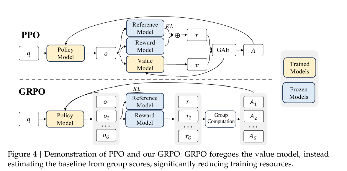
Figure 4. PPO와 GRPO 구조 비교

Figure 4는 PPO와 GRPO의 차이를 가장 직관적으로 보여준다.

PPO에서는 하나의 output을 생성한 뒤 Reward Model과 Value Model을 사용한다.

Question
   ↓
Policy Model
   ↓
Output
   ├─ Reward Model
   ├─ Reference Model
   └─ Value Model
          ↓
     Reward + Value
          ↓
         GAE
          ↓
      Advantage

반면 GRPO에서는 Value Model을 사용하지 않는다.

하나의 question에 대해 여러 개의 response를 sampling한다.

o_1,o_2,\dots,o_G

각 response에 reward를 부여한다.

r_1,r_2,\dots,r_G

그리고 같은 question에서 생성된 response들의 reward를 서로 비교하여 advantage를 계산한다.

Question
   ↓
Policy Model
   ↓
o1, o2, ..., oG
   ↓
r1, r2, ..., rG
   ↓
Group Computation
   ↓
A1, A2, ..., AG

즉 핵심 변화는 다음과 같다.

\boxed{ \text{PPO: Value Model + GAE} \quad\longrightarrow\quad \text{GRPO: Group-relative Advantage} }

Value Model 자체를 학습하지 않아도 되므로 training resource를 줄일 수 있다.

6. GRPO Objective

GRPO는 Value Model을 제거하지만, PPO의 clipped policy update 자체를 버리는 것은 아니다.

GRPO objective는 다음과 같다.

J_{\mathrm{GRPO}}(\theta) = \mathbb{E} \left[ \frac{1}{G} \sum_{i=1}^{G} \frac{1}{|o_i|} \sum_{t=1}^{|o_i|} \left( \min \left( \rho_{i,t}\hat A_{i,t}, \operatorname{clip} \left( \rho_{i,t}, 1-\epsilon, 1+\epsilon \right) \hat A_{i,t} \right) - \beta D_{\mathrm{KL}} [ \pi_\theta\|\pi_{\mathrm{ref}} ] \right) \right]

처음 보면 복잡하지만 크게 세 부분만 보면 된다.

Policy Ratio

\rho_{i,t} = \frac{ \pi_\theta(o_{i,t}\mid q,o_{i,<t}) }{ \pi_{\theta_{\mathrm{old}}}(o_{i,t}\mid q,o_{i,<t}) }

old policy 대비 current policy의 token probability 변화를 나타낸다.

Group-relative Advantage

\hat A_{i,t}

PPO처럼 Value Model에서 계산하는 것이 아니라, 같은 question에서 생성된 여러 response의 relative reward를 이용해 계산한다.

KL Regularization

D_{\mathrm{KL}} [ \pi_\theta\|\pi_{\mathrm{ref}} ]

current policy가 reference policy에서 과도하게 divergence하는 것을 제한한다.

따라서 GRPO objective는 크게 다음과 같이 볼 수 있다.

\boxed{ \text{PPO-style Clipping} + \text{Group-relative Advantage} + \text{KL Regularization} }

7. GRPO에서는 KL을 어떻게 사용할까?

PPO에서는 KL-related penalty를 reward 안에 포함시켰다.

반면 GRPO에서는 KL divergence를 objective에 직접 regularization term으로 추가한다.

GRPO에서는 다음 unbiased estimator를 사용한다.

D_{\mathrm{KL}} [ \pi_\theta\|\pi_{\mathrm{ref}} ] = \frac{ \pi_{\mathrm{ref}}(o_{i,t}\mid q,o_{i,<t}) }{ \pi_\theta(o_{i,t}\mid q,o_{i,<t}) } - \log \frac{ \pi_{\mathrm{ref}}(o_{i,t}\mid q,o_{i,<t}) }{ \pi_\theta(o_{i,t}\mid q,o_{i,<t}) } -1

비율을

x = \frac{\pi_{\mathrm{ref}}}{\pi_\theta}

라고 하면

x-\log x-1

형태이며,

x-\log x-1 \ge 0

이므로 non-negative가 보장된다.

정리하면,

PPO
KL-related penalty
→ reward 내부에 포함
→ Advantage 계산에도 영향

GRPO
Group reward
→ Advantage 계산

KL divergence
→ objective에 별도 regularization

즉 relative reward를 이용한 advantage estimation과 KL regularization을 분리한다.

8. Outcome Supervision

그렇다면 group의 reward를 token-level Advantage로 어떻게 바꿀까?

첫 번째 방법은 Outcome Supervision이다.

하나의 question에 대해 생성된 G개의 response reward를

\mathbf{r} = \{r_1,r_2,\dots,r_G\}

라고 하자.

각 reward를 group 내부에서 normalize한다.

\bar r_i = \frac{ r_i-\operatorname{mean}(\mathbf r) }{ \operatorname{std}(\mathbf r) }

Outcome Supervision에서는 output 하나의 모든 token에 동일한 Advantage를 부여한다.

\hat A_{i,t} = \bar r_i

예를 들어 한 response의 normalized reward가

+1.2

라면,

Token 1  → +1.2
Token 2  → +1.2
Token 3  → +1.2
...
Token T  → +1.2

가 된다.

즉 최종 outcome이 좋았다면 해당 response 전체를 동일하게 reinforce한다.

구조가 단순하지만, reasoning 과정에서 어느 step이 좋았고 어느 step이 잘못되었는지는 구분하기 어렵다.

9. Process Supervision

Process Supervision은 response 전체에 reward 하나를 주는 대신 reasoning step별로 reward를 제공한다.

j번째 reasoning step의 마지막 token index를

\operatorname{index}(j)

라고 하면 각 step reward를 normalize하여 다음과 같이 표현할 수 있다.

\bar r_i^{\operatorname{index}(j)} = \frac{ r_i^{\operatorname{index}(j)} - \operatorname{mean}(R) }{ \operatorname{std}(R) }

그리고 token t의 Advantage는 현재 token 이후에 존재하는 reasoning step들의 normalized reward의 합으로 계산한다.

\hat A_{i,t} = \sum_{\operatorname{index}(j)\ge t} \bar r_i^{\operatorname{index}(j)}

즉 차이는 다음과 같다.

Outcome Supervision

Response
   ↓
Final Reward 하나
   ↓
모든 token에 동일한 Advantage

Process Supervision

Reasoning Step 1 → Reward
Reasoning Step 2 → Reward
Reasoning Step 3 → Reward
        ↓
token별로 더 세밀한 Advantage

따라서 Process Supervision은 Outcome Supervision보다 credit assignment의 granularity가 더 높다.

10. Iterative GRPO

RL이 진행되면 policy의 output distribution도 계속 바뀐다.

그러면 초기 policy를 기반으로 학습된 Reward Model이 현재 policy의 output을 계속 정확하게 평가한다고 보장하기 어렵다.

그래서 DeepSeekMath는 iterative RL도 사용한다.

Current Policy
      ↓
새 Response Sampling
      ↓
Reward Model용 새 Data 생성
      ↓
Reward Model Update
      ↓
Policy Update
      ↓
Repeat

Reward Model을 계속 새로운 data로만 학습하면 이전 정보를 잊을 수 있으므로, historical data의 10%를 포함한 replay mechanism도 사용한다.

실험에서는 iterative RL이 추가적인 성능 향상을 보였으며, 특히 첫 번째 iteration에서 큰 향상이 나타났다.

11. GRPO를 더 일반적인 관점에서 보기

논문에서는 SFT, RFT, DPO, PPO, GRPO를 완전히 별개의 방법으로만 보지 않고, 하나의 unified paradigm으로 분석한다.

일반적인 training method의 gradient를 다음처럼 표현한다.

\nabla_\theta J_A(\theta) = \mathbb{E}_{(q,o)\sim D} \left[ \frac{1}{|o|} \sum_{t=1}^{|o|} GC_A(q,o,t,\pi_{rf}) \nabla_\theta \log \pi_\theta(o_t\mid q,o_{<t}) \right]

여기서 중요한 요소는 세 가지다.

Data Source

어떤 training sample을 사용할 것인가.

Reward Function

어떤 기준으로 response의 quality를 판단할 것인가.

Algorithm

data와 reward signal을 실제 Gradient Coefficient로 어떻게 변환할 것인가.

즉,

\boxed{ \text{Data Source} + \text{Reward Function} + \text{Algorithm} \rightarrow \text{Gradient Coefficient} }

라는 관점이다.

12. RFT, Online RFT, GRPO의 차이

이 unified view에서 GRPO의 효과를 조금 더 명확하게 볼 수 있다.

RFT

SFT model에서 여러 response를 생성하고, 정답인 response만 남겨 다시 supervised fine-tuning한다.

Response Sampling
      ↓
Correctness Filtering
      ↓
Correct Response만 학습

즉 incorrect response는 penalize하는 것이 아니라 단순히 버린다.

Online RFT

RFT와 비슷하지만 response를 초기 SFT model이 아니라 현재 policy에서 계속 새로 sampling한다.

Current Policy
      ↓
새 Response Sampling
      ↓
Correct Response Filtering
      ↓
Fine-tuning

현재 policy가 변화할수록 최신 policy distribution을 반영할 수 있다는 장점이 있다.

GRPO

GRPO 역시 current policy에서 response를 sampling하지만, 단순히 correct / incorrect로 filtering하지 않는다.

Relative reward에 따라 reinforcement 강도를 다르게 적용한다.

높은 Relative Reward
→ Strong Reinforcement

조금 높은 Reward
→ Weak Reinforcement

낮은 Relative Reward
→ Penalization

즉 Online RFT와 GRPO의 중요한 차이는:

\boxed{ \text{Filtering} \quad\text{vs}\quad \text{Reward-weighted Gradient Update} }

이다.

13. 실제로 GRPO가 더 효과적이었을까?

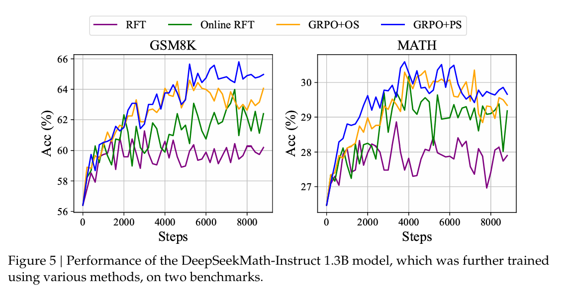
Figure 5. RFT, Online RFT, GRPO+OS, GRPO+PS 비교

Figure 5에서는 크게 두 가지를 확인할 수 있다.

첫째, Online RFT가 RFT보다 좋은 성능을 보인다.

초기에는 current policy와 SFT model이 비슷하기 때문에 차이가 크지 않지만, training이 진행될수록 두 policy의 distribution이 달라진다.

따라서 후반에는 current policy에서 직접 sampling하는 online 방식의 이점이 커진다.

둘째, GRPO가 Online RFT보다 더 좋은 성능을 보인다.

Online RFT는 correct response를 동일한 강도로 reinforce하고 incorrect response는 버린다.

반면 GRPO는 relative reward에 따라 positive / negative gradient coefficient의 크기를 다르게 적용한다.

또한 GRPO+PS가 GRPO+OS보다 더 높은 성능을 보이는 경향은 step-aware한 fine-grained supervision이 도움이 될 수 있음을 보여준다.

14. Why Does RL Work?

논문의 Discussion에서 흥미로운 분석 중 하나는 Pass@K와 Maj@K의 비교이다.

Pass@K

K개의 candidate를 생성했을 때, 그중 정답이 하나라도 존재하는지 측정한다.

즉 모델이 correct solution을 생성할 capability를 가지고 있는지를 보는 데 가깝다.

Maj@K

K개의 candidate 중 가장 많이 등장한 answer가 정답인지 측정한다.

즉 sampling을 반복했을 때 정답으로 얼마나 일관되게 수렴하는지 본다.

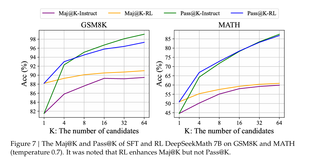
Figure 7. SFT와 RL model의 Maj@K / Pass@K 비교

실험 결과 RL 이후

\text{Maj@K} \uparrow

했지만,

\text{Pass@K}

는 크게 향상되지 않았다.

이 결과는 꽤 중요한 의미를 가진다.

SFT model도 여러 candidate를 충분히 sampling하면 이미 correct response를 생성할 수 있었다.

즉 RL 이후 완전히 새로운 solution을 생성할 수 있게 되었다기보다는,

기존 Top-K 안에 존재하던 correct response가 더 높은 probability를 갖도록 output distribution이 조정되었다

고 볼 수 있다.

논문에서는 이를 RL이 output distribution을 더 robust하게 만든 것으로 해석한다.

즉 RL의 효과는 단순히

\text{New Capability Acquisition}

만으로 설명하기보다는,

\text{Existing Capability} \rightarrow \text{Better Alignment} \rightarrow \text{Correct Response Probability 증가}

의 관점에서도 볼 수 있다.

15. 더 효과적인 RL을 위해서는?

Data Source

이 논문에서는 기존 instruction tuning question과 비교적 단순한 nucleus sampling을 사용했다.

저자들은 이것이 Pass@K가 크게 향상되지 않은 이유 중 하나일 수 있다고 본다.

향후에는

Out-of-Distribution question
advanced decoding
tree-search 기반 exploration

등을 활용하여 더 다양한 reasoning trajectory를 탐색할 필요가 있다고 제안한다.

Algorithm

현재 RL algorithm은 reward signal을 상당히 강하게 신뢰한다.

하지만 Reward Model이나 human annotation 역시 오류를 포함할 수 있다.

따라서 앞으로는 noisy reward signal에도 robust한 RL algorithm이 중요하다고 본다.

이는 weak supervisor를 이용해 더 강한 model을 학습하는 Weak-to-Strong alignment와도 연결된다.

Reward Function

Reward Model에서는 크게 세 가지 방향을 제시한다.

OOD input과 새로운 decoding output에 대한 generalization
Reward Model의 uncertainty 반영
reasoning 과정에 fine-grained signal을 제공하는 high-quality Process Reward Model

특히 세 번째 방향은 앞서 GRPO+PS가 보여준 결과와도 연결된다.

16. 정리

GRPO의 핵심은 PPO를 완전히 새로운 algorithm으로 대체하는 것이 아니다.

PPO의 policy ratio와 clipping 기반 update 구조는 유지하면서, 가장 큰 변화는 Advantage를 계산하는 방식에 있다.

PPO에서는

\text{Reward} + \text{Value Model} \rightarrow \text{GAE} \rightarrow \text{Advantage}

를 사용한다.

반면 GRPO에서는

\text{Multiple Responses} \rightarrow \text{Relative Rewards} \rightarrow \text{Group-relative Advantage}

를 사용한다.

따라서 GRPO를 다음과 같이 요약할 수 있다.

\boxed{ \text{GRPO} = \text{PPO-style Clipped Optimization} + \text{Group-relative Advantage} - \text{Value Model} }

Value Model을 제거함으로써 memory와 computation cost를 줄이고, 같은 question에 대한 여러 response의 relative reward를 이용하여 policy를 학습한다.

또한 DeepSeekMath의 실험에서는

offline보다 online sampling이 효과적이었고
단순 rejection보다 reward magnitude를 gradient에 직접 반영하는 것이 효과적이었으며
Process Supervision이 finer-grained credit assignment를 제공했고
iterative RL을 통해 Reward Model 역시 현재 policy에 맞춰 갱신할 수 있었다.

마지막으로 Pass@K와 Maj@K 분석은 RL의 역할을 조금 다르게 바라보게 한다.

RL은 반드시 완전히 새로운 reasoning capability를 만들어내는 것만이 아니라, 이미 model 내부에 존재하는 좋은 response를 더 높은 확률로 선택하도록 policy distribution을 정렬하는 과정으로도 볼 수 있다.

onpo

다음 포스트

DeepSeekMath: Pushing the Limits of Mathematical Reasoning in Open Language Models (24.02)

Paper Notes

DeepSeekMath: GRPO 이해하기

1. DeepSeekMath는 어떤 모델인가?

2. PPO부터 이해하기

2.1 PPO에서 clipping을 사용하는 이유

3. PPO에서 Advantage는 어떻게 계산할까?

4. PPO에서 Reward와 KL Penalty

5. PPO에서 GRPO로

6. GRPO Objective

Policy Ratio

Group-relative Advantage

KL Regularization

7. GRPO에서는 KL을 어떻게 사용할까?

8. Outcome Supervision

9. Process Supervision

10. Iterative GRPO

11. GRPO를 더 일반적인 관점에서 보기

Data Source

Reward Function

Algorithm

12. RFT, Online RFT, GRPO의 차이

RFT

Online RFT

GRPO

13. 실제로 GRPO가 더 효과적이었을까?

14. Why Does RL Work?

Pass@K

Maj@K

15. 더 효과적인 RL을 위해서는?

Data Source

Algorithm

Reward Function

16. 정리

Neural Discrete Representation Learning

0개의 댓글