CS231N, EECS 498-007 / 598-005에서 나타나는 개념을 정리하기 위하여 복기용도로 작성하였습니다.
간단히 정리한 내용을 살펴보며 모르는 부분이 있을 때 찾아보는 용도로 보시면 좋을 것 같습니다.
Recurrent Neural Networks: Process Sequences
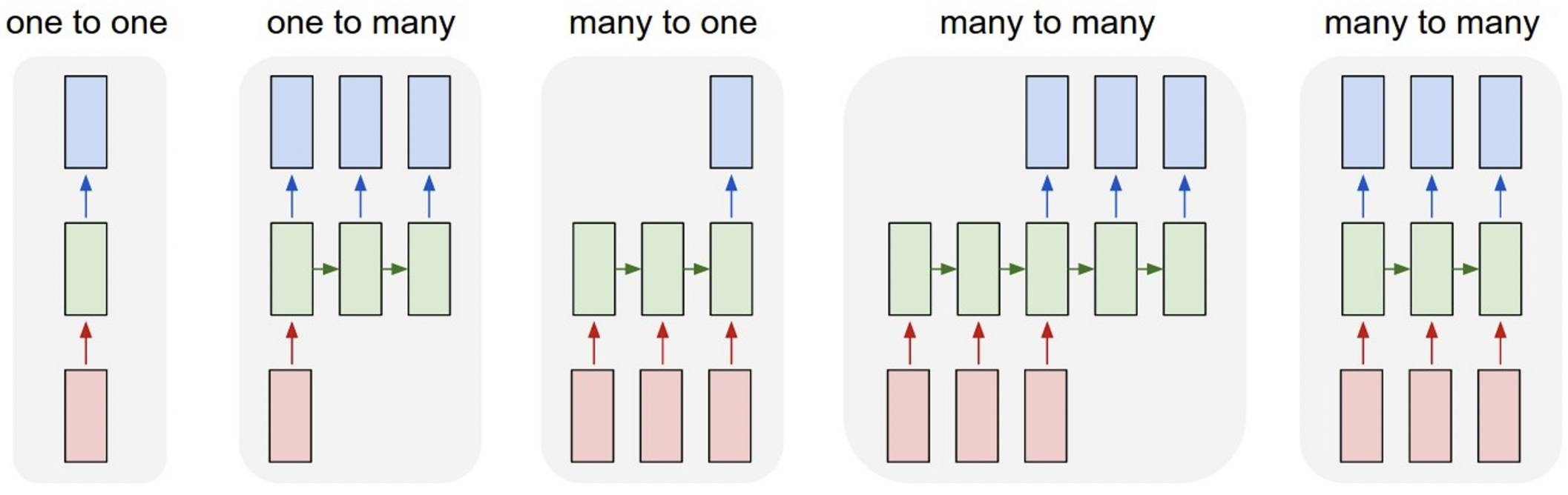
- Single input & Single output
Image classification: Image -> Label - Single input & Sequence output
Image Captioning: Image -> sequence of words - Sequence input & Single output
Video classification: Sequence of images -> label - Sequence input & Sequence output
Machine Translation: Sequence of words -> Sequence of words - Sequence input & Sequence output
Per-frame video classification: Sequence of images -> Sequence of labels
Recurrent Neural Networks
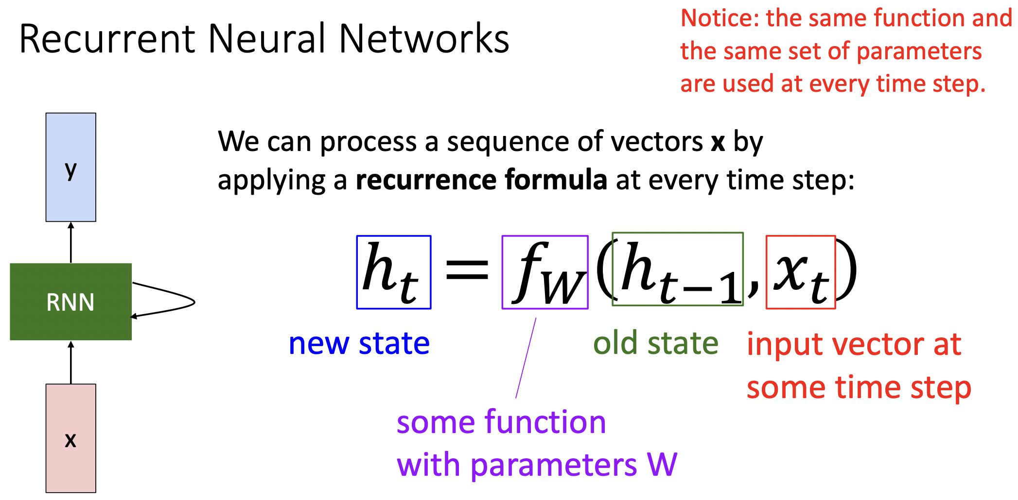
- RNN은 입력값으로 x을 받은다음 출력값으로 y와 sequence가 처리될때마다 업데이트하는 internal hidden state(벡터)가 존재한다.
- 는 t시간 일때의 hidden state으로 함수 는 파라미터 (직전 시간의 hidden state)와 (t시간일 때의 입력값)를 필요로 한다.
- 는 모든 시간 및 sequence에서 동일한 weight matrix를 가진다.
(Vanilla) Recurrent Neural Networks
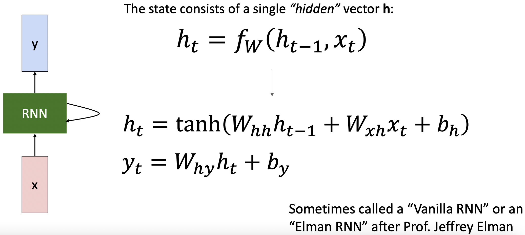
- 각 파리미터에 해당하는 weight matrix를 곱한뒤 tanh를 적용하면 현 시점의 hidden state를, 현 시점의 hidden state에 weight matrix를 곱하면 현 시점의 output 를 얻을 수 있다.
RNN Computational Graph
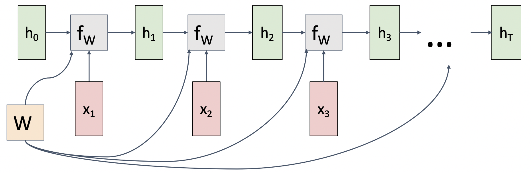
- 동일한 weight matrix를 매 time-step마다 사용하여 arbitrary한 sequence라도 처리가 가능하다.
RNN Computational Graph (Many to Many)
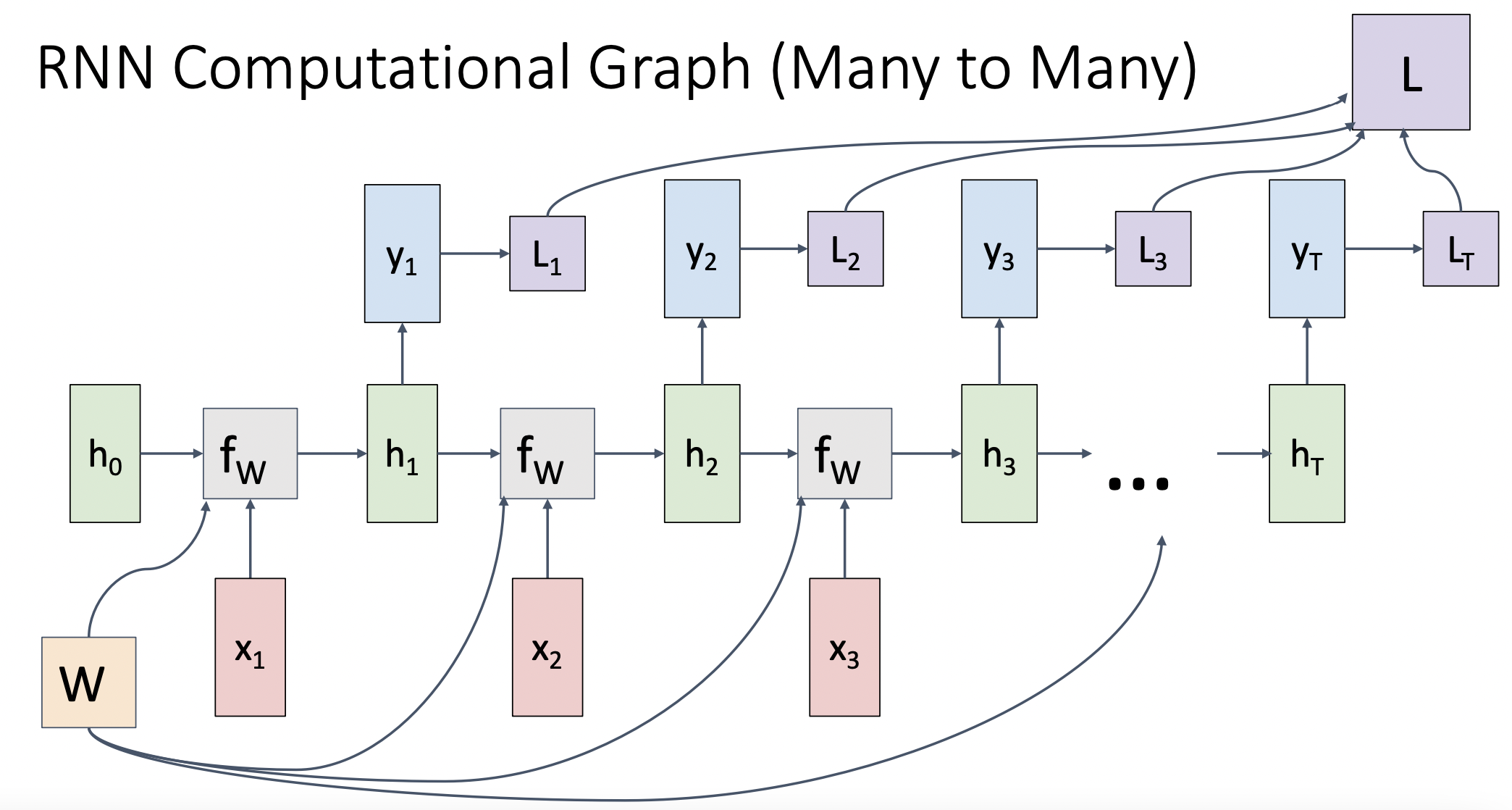
- 매 time-step의 출력 값에 loss를 적용하여 각 시간대의 분류문제를 적용 하고 총 결과를 종합할 수 있다.
RNN Computational Graph (Many to One)
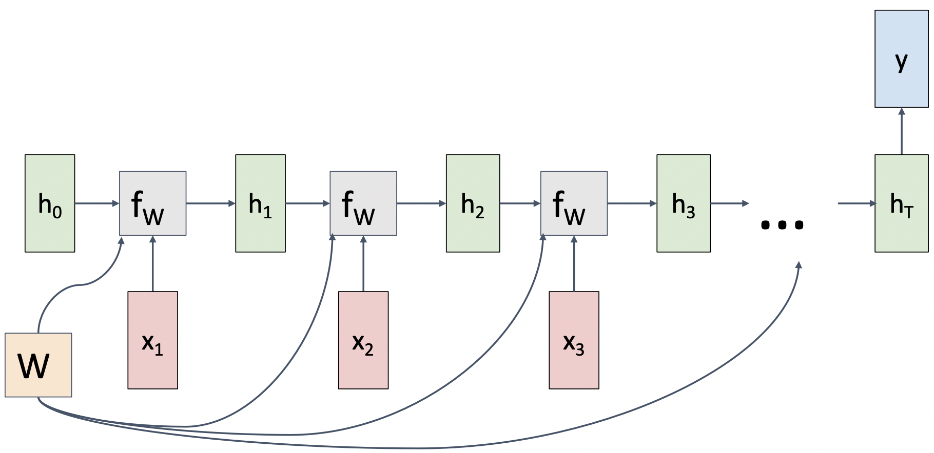
- video CLF같은 경우 다음과 같이 마지막 sequence만 확인한다.
Sequence to Sequence (seq2seq)
(Many to one) + (One to many)
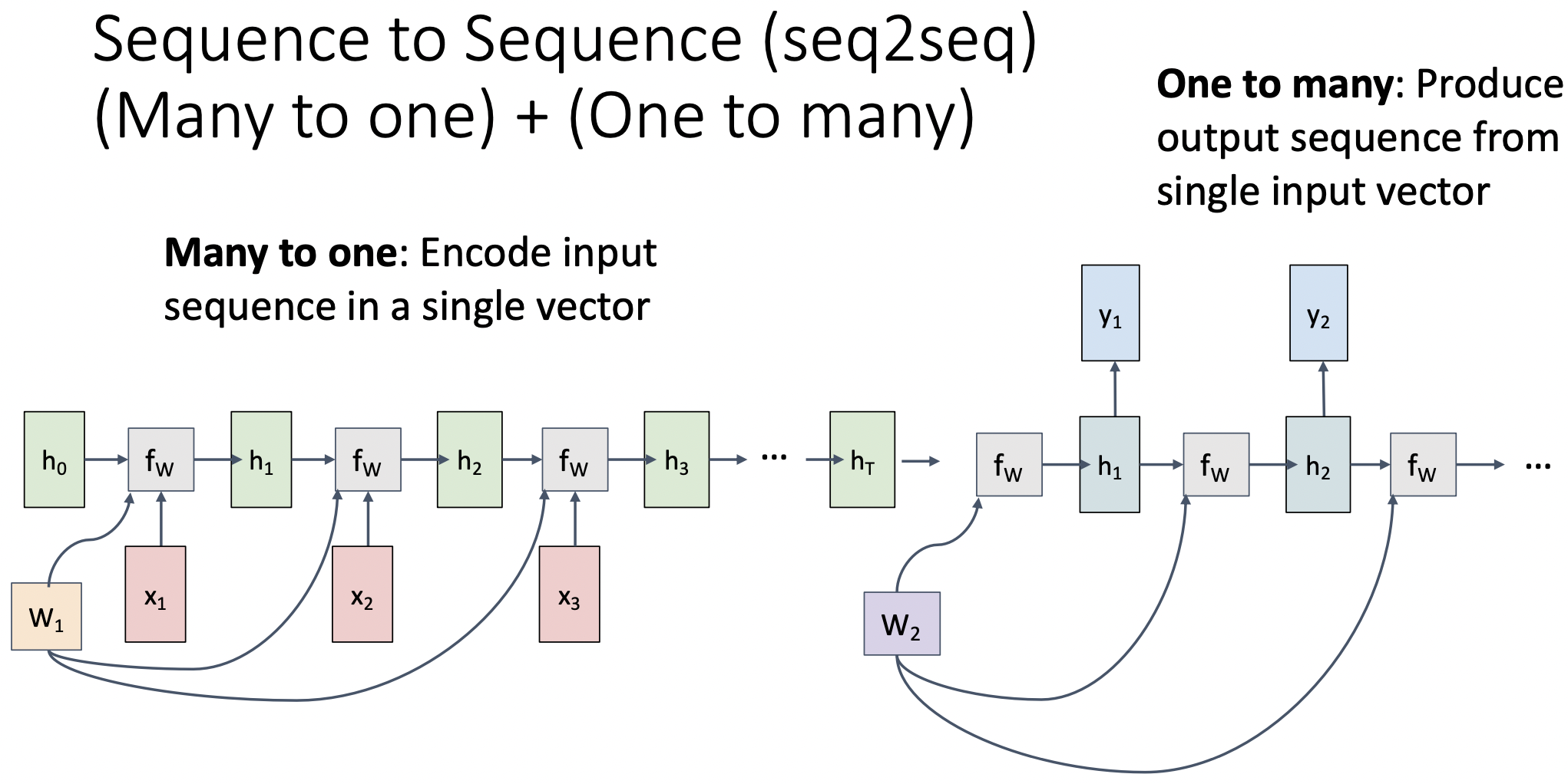
- machine translation의 경우 출력값의 순서와 길이가 다를 수 있다.
- 입력 값을 encode한 뒤, encode된 벡터를 두번째 rnn에(decoder) 입력으로 넣는다.
- encoder: many to one
- decoder: one to many
Example: Language Modeling
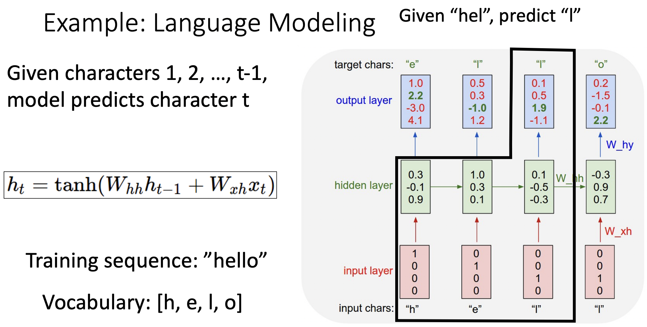
- input chars을 원 핫 형식으로 지정한다음 예측 값으로는 순차적인 다음 글자를 찾는 모델이다. ("hell" => "ello")
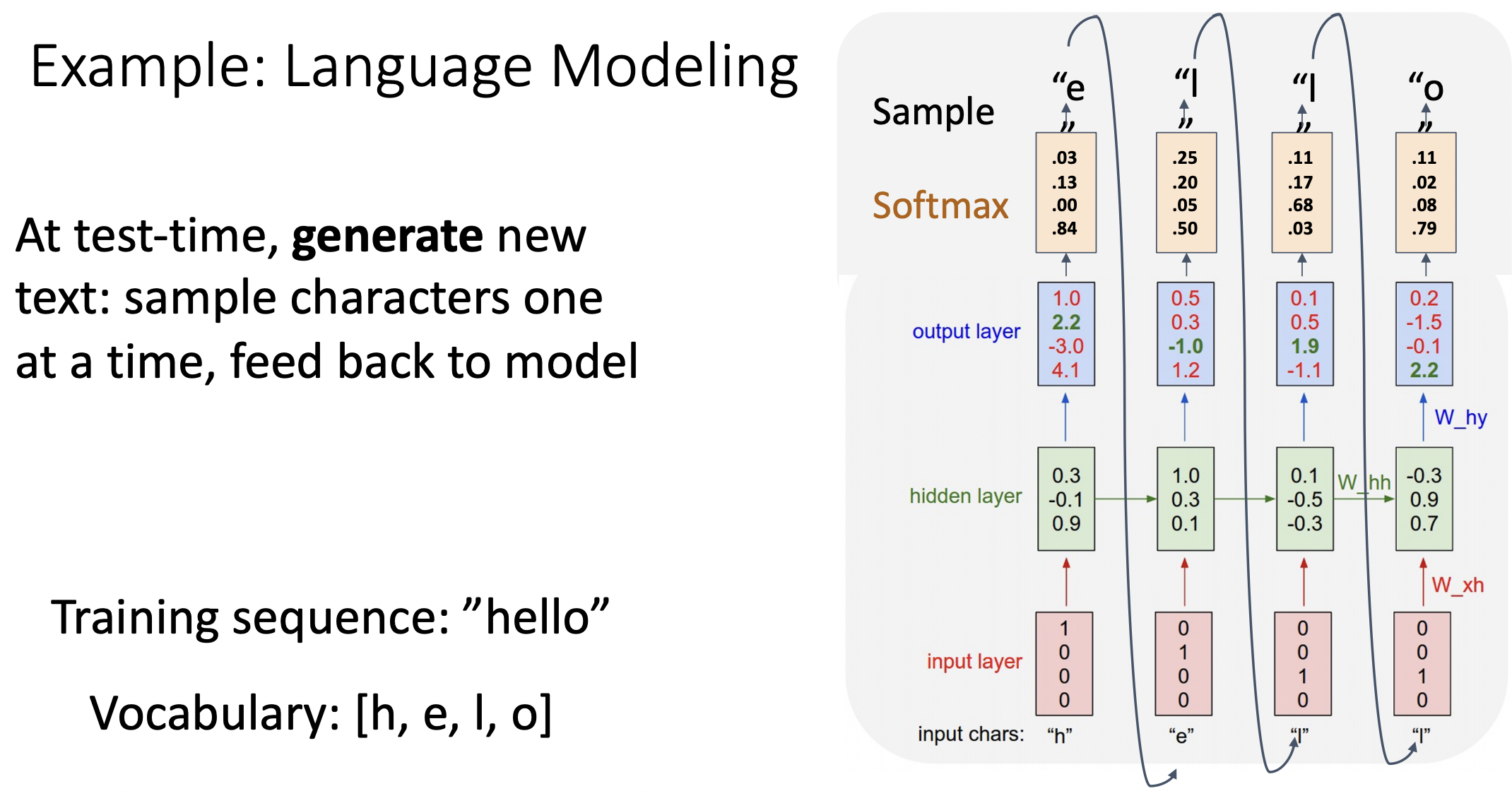
- test time에서는 각 단계에서 예측한 값을 다음 단계의 입력값으로 사용한다.
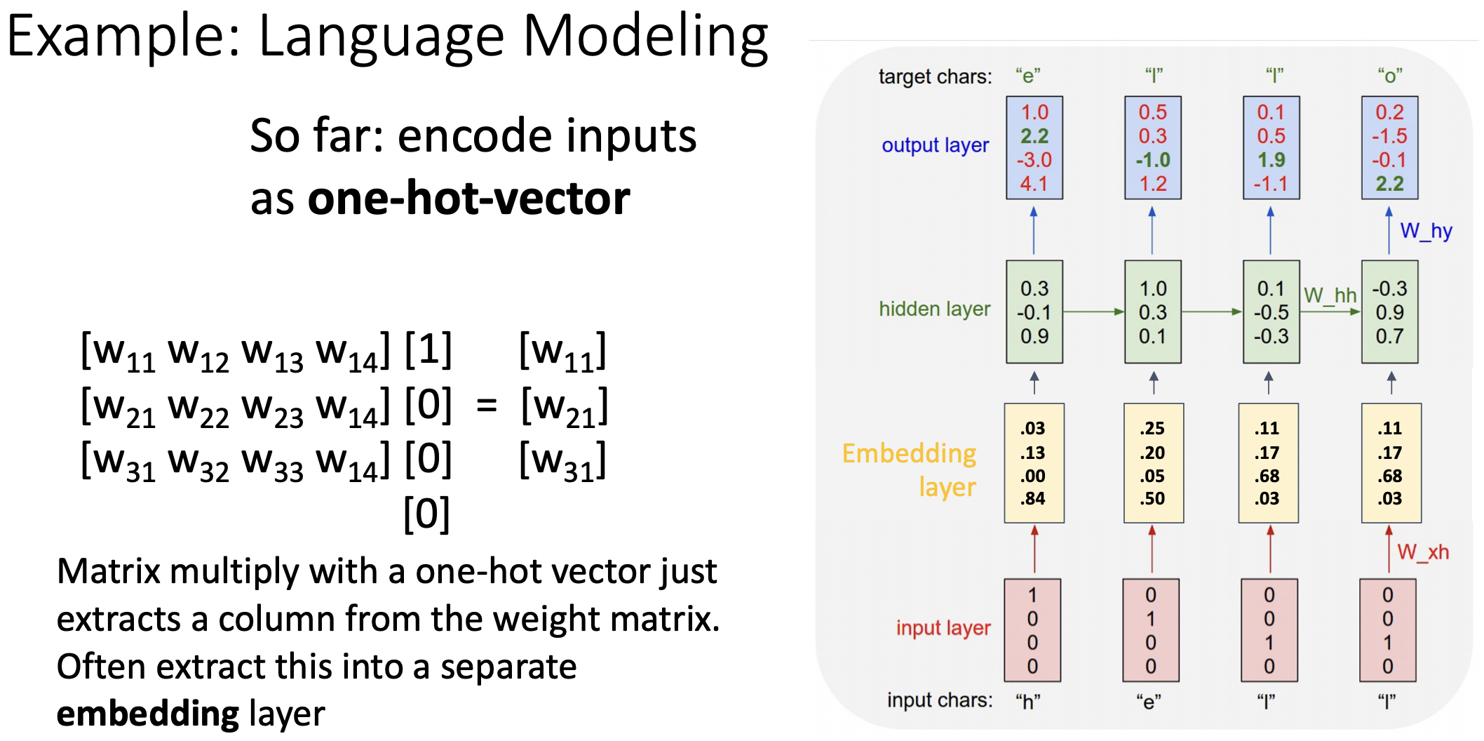
- 보통 원 핫 형식의 입력값을 바로 sequence model에 넣지 않고 embbeding layer을 거친다.
Truncated Backpropagation Through Time
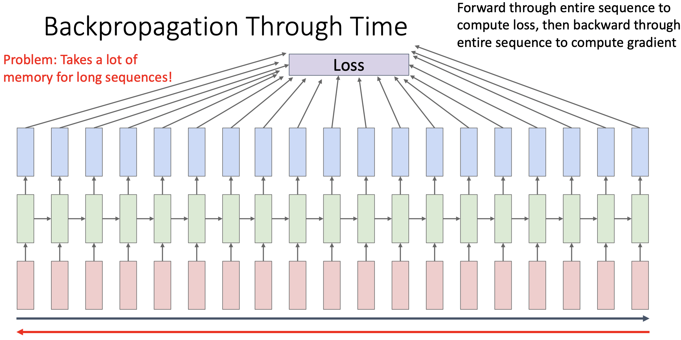
- P: sequence가 긴 모델의 경우 많은 양의 메모리가 필요하다.
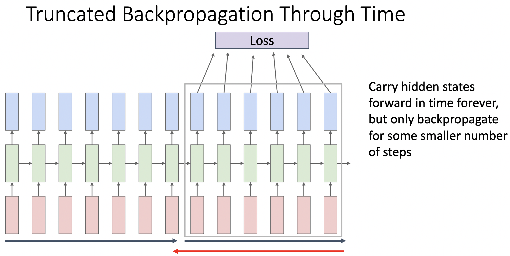
- S: 전체 sequence를 다 수행하지 않고 sequence를 나누어 학습을 진행한다.
이전 단계chunk에서 학습한 weight를 사용하여 다음 chunk를 학습한다.
Searching for Interpretable Hidden Units
- RNN의 각 hidden state가 어떤의미를 지니는지 다양한 텍스트와 여러 단계의 hidden state를 사용하여 분석해본다.
- hidden state의 output은 tanh를 지나 -1에서 1사이의 값을 가진다.
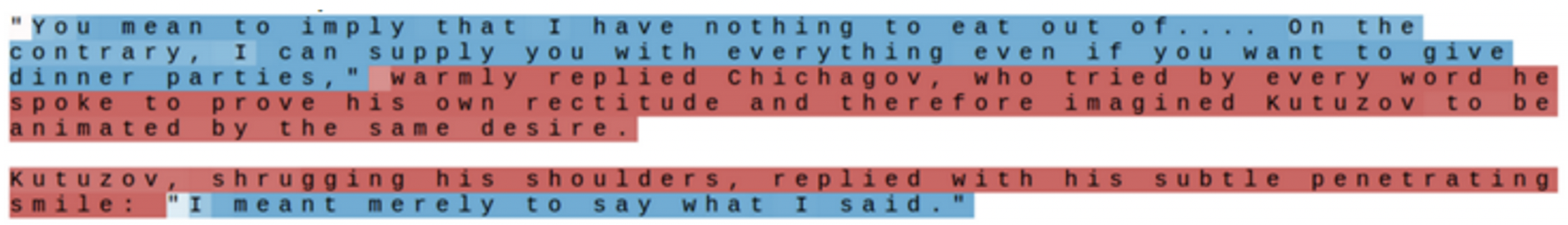
- 따옴표의 상대적 위치를 구분하는 hidden state
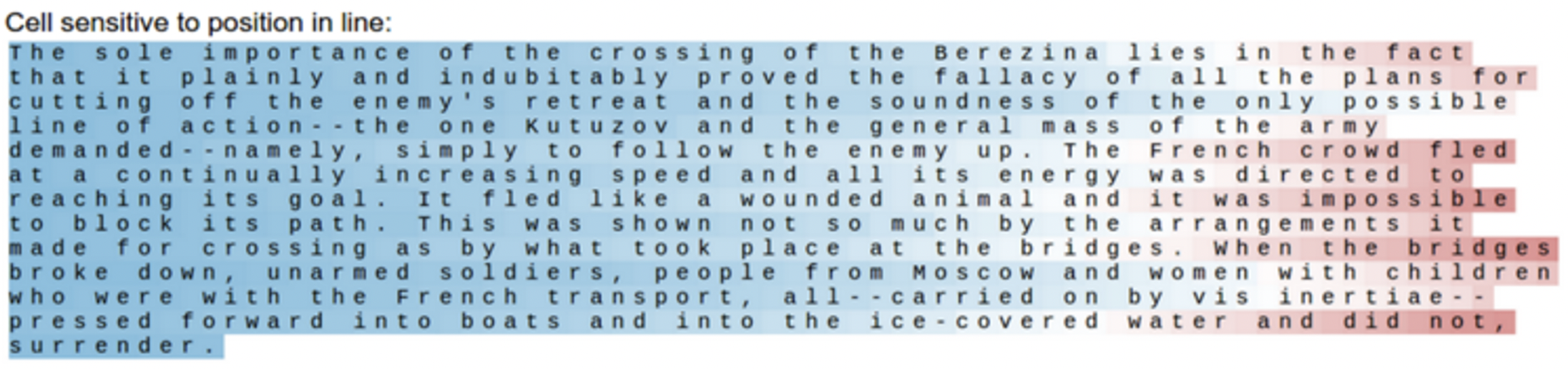
- 글자의 상대적 위치를 구분하는 hidden state
- 코드의 깊이를 구분하는 hidden state
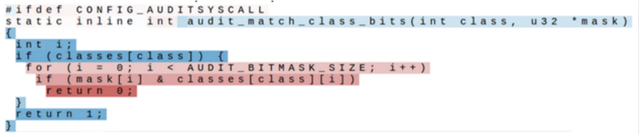
- 위의 사례를 통해 각각의 hidden state의 activation은 특정 feature를 찾아내는 기능을 한다.
Example: Image Captioning
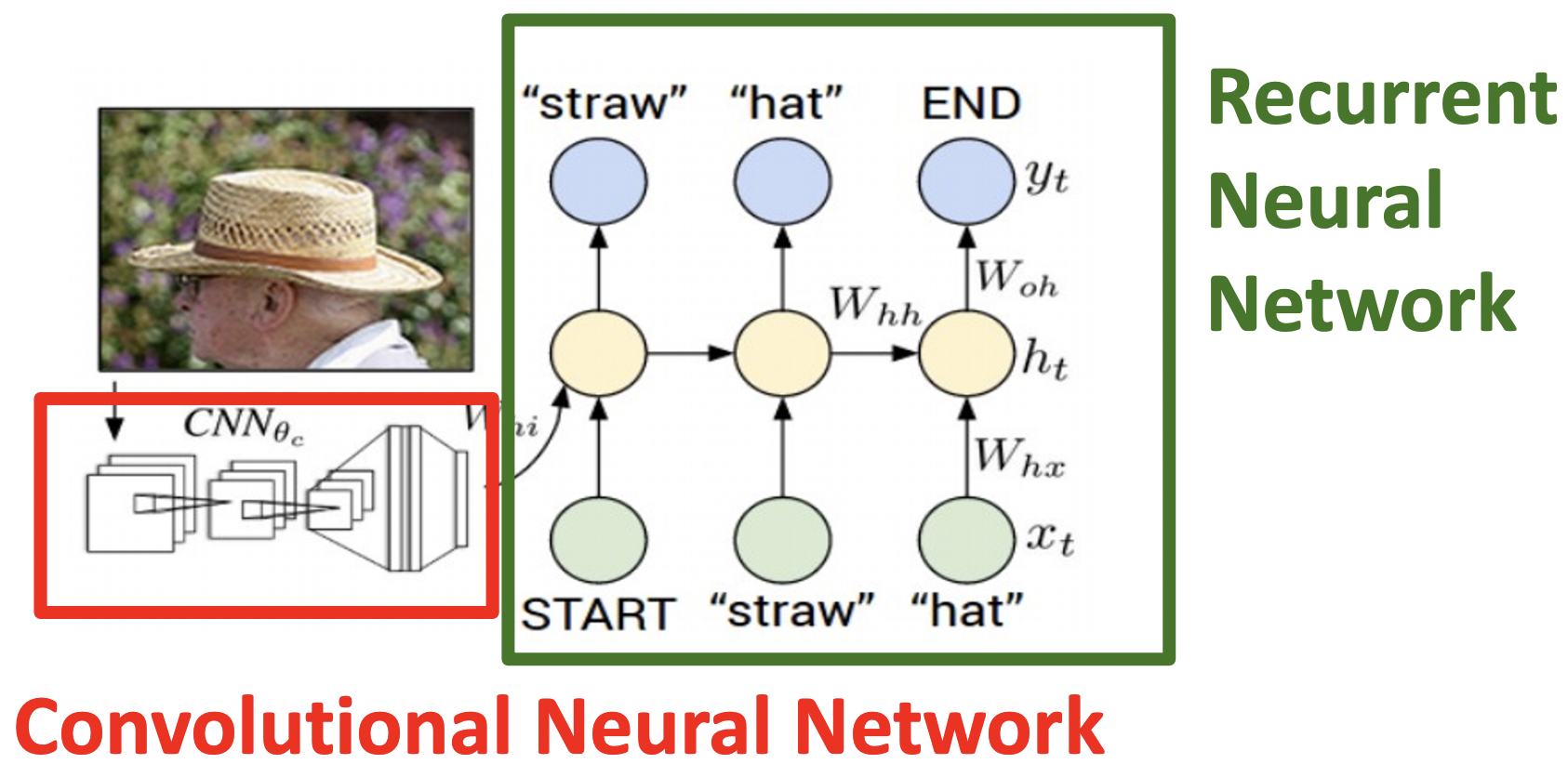
- pretrain 된 모델의 feature를 RNN의 입력 값에 추가하여 Image Captioning에 사용했다.
Vanilla RNN Gradient Flow
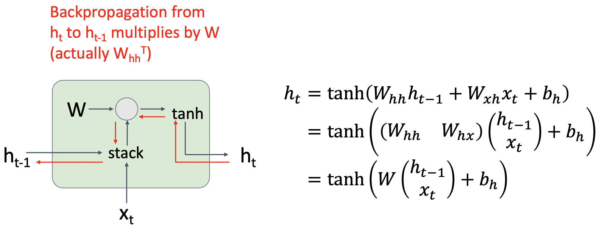
- 파란색은 forward pass이며, 빨간색은 backward pass이다.
- P1: back propagation시 tanh에서 vanishing gradinent 문제가 발생한다.
- P2: back propagation시 weight matrix의 Transpose를 연속하여 곱하는데 exploding gradinent와 vanishing gradinent 문제가 발생한다.
- weight matrix의 Transpose를 거듭제곱 형태로 나타내는데 이를 eigen decomposition 과정을 통해 singular value의 거듭제곱 형태로 나타낼 수 있다.
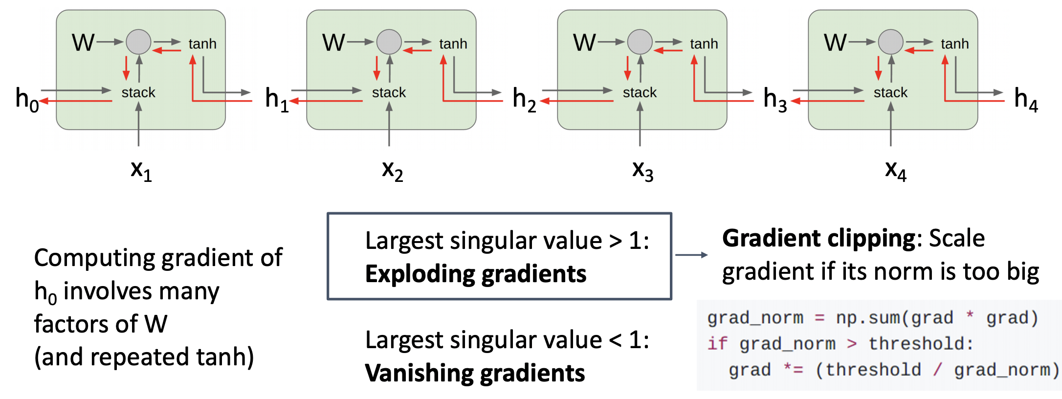
- Largest singular value > 1 라면 gradient clipping : gradient가 너무 커지지 않게 scaling
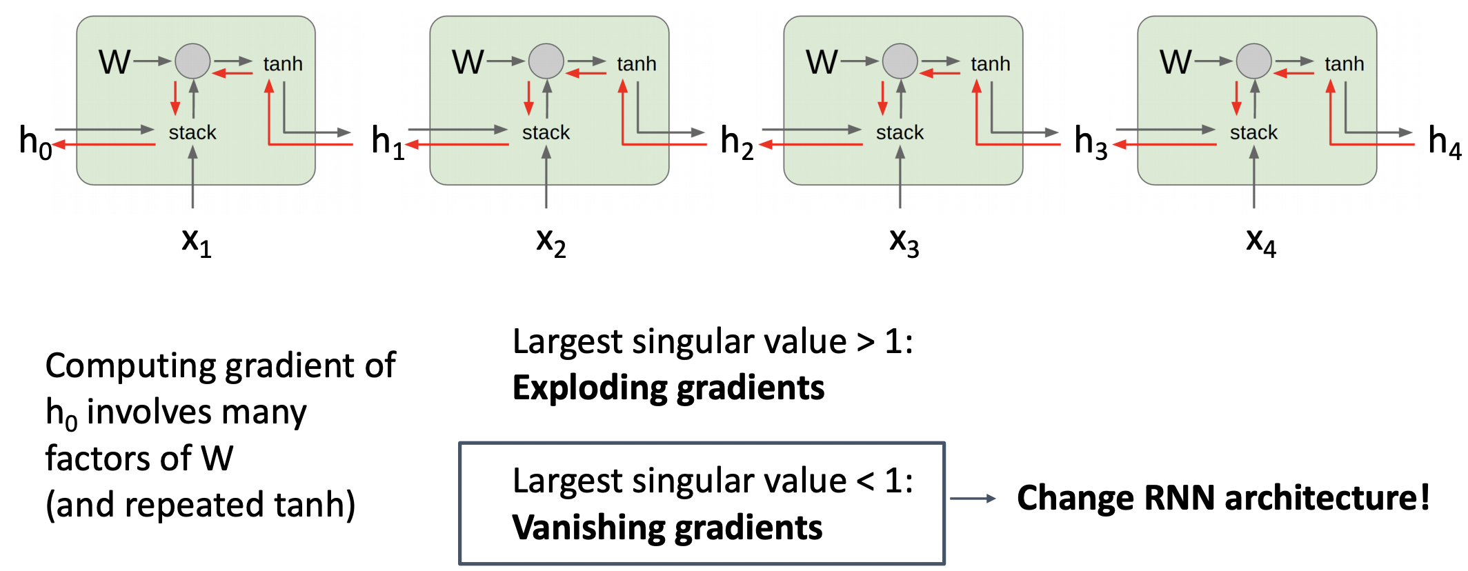
- Largest singular value < 1 라면 change RNN
Long Short Term Memory (LSTM)
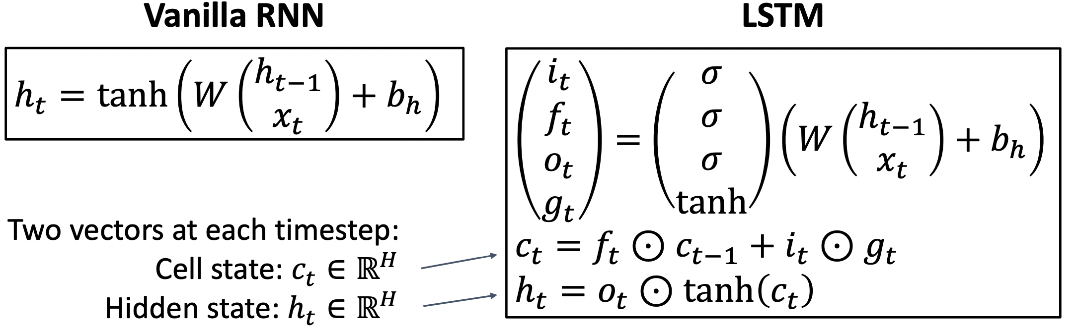
- 두개의 hidden vector인 Cell state vector:와 Hidden state vector:를 가진다.
- input value와 hiden state value를 통해 4가지의 gate value를 매 state마다 계산한다.
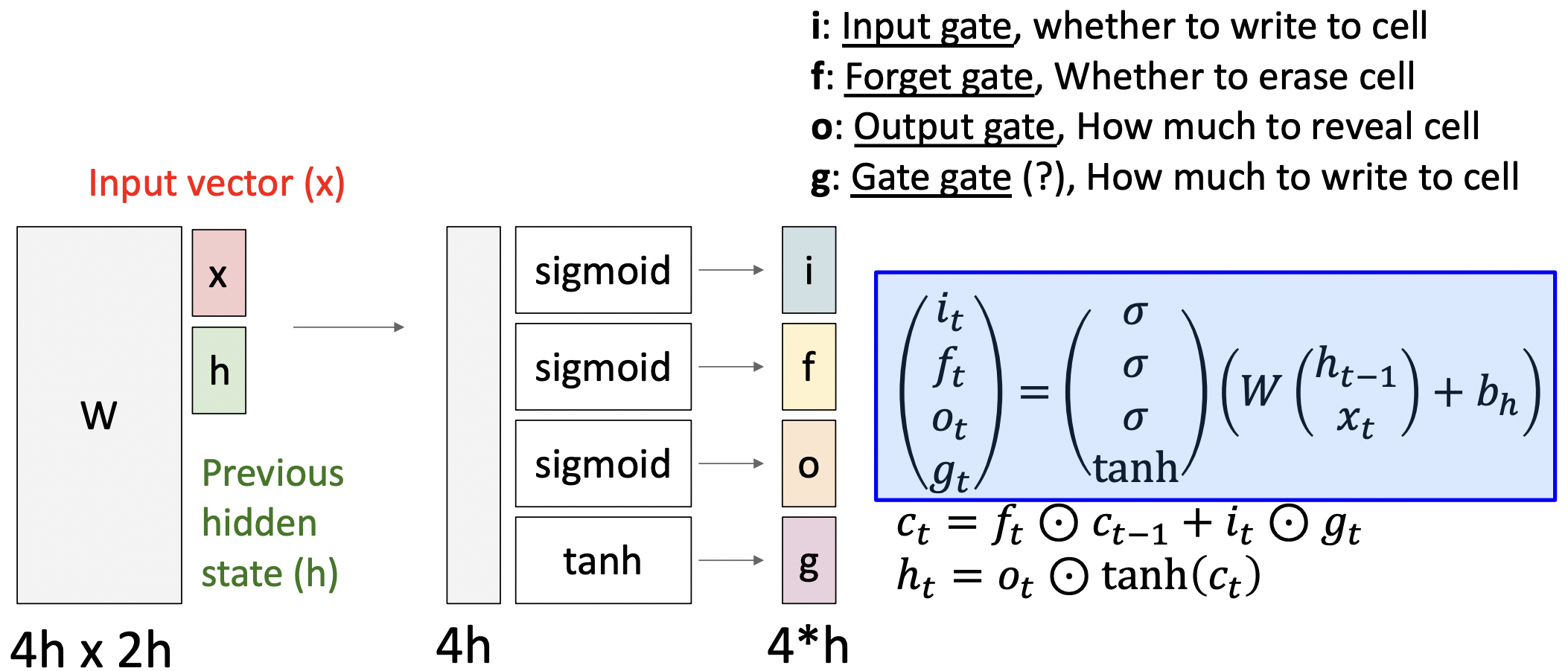
- input value와 hiden state value를 가지고 바로 hiden state value를 계산하지 않고 여러가지의 gate value를 통해 간접적으로 계산한다.
- Cell state vector 계산시 직전 Cell state vector를 얼마나 반영할지 forget gate(0~1)를 곱해주고 새로운 입력 값을(input gate, 0~1) 어떻게 반영할지(gate gate, -1~+1) 더해준다.
- Cell state vector는 결국 내부 hiden state를 나타내며 이를 output gate가 조정한다.
Long Short Term Memory (LSTM): Gradient Flow
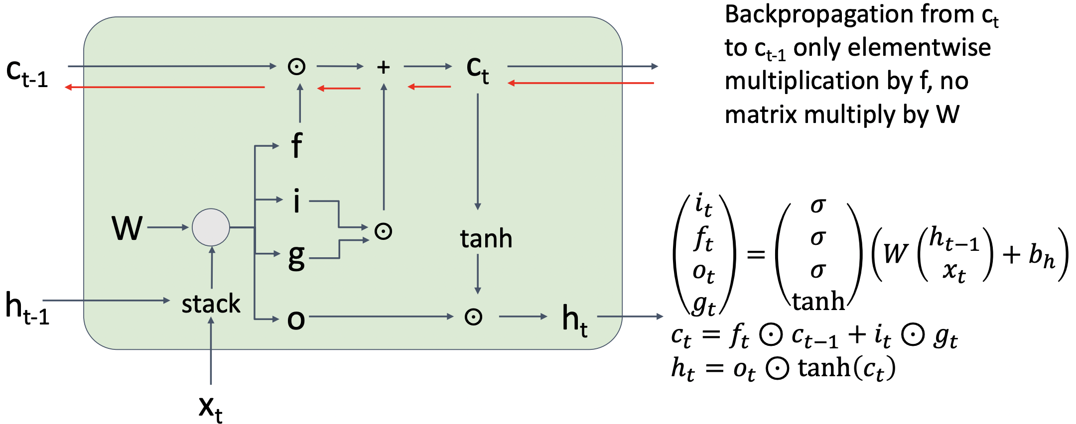
- Cell state vector계산시에 Weight matrix의 거듭제곱 형태가 아닌 elementwise multiplication 형태로 나타낼 수 있다.
- 따라서 직접적인 weight matrix의 영향을 받지 않고 non-linearity형태를 직접적으로 통과하지 않기 때문에 RNN보다 나은 학습이 가능하다.
- 하지만 forget gate가 0에 가깝다면 학습 진행이 어려울 수 있다.
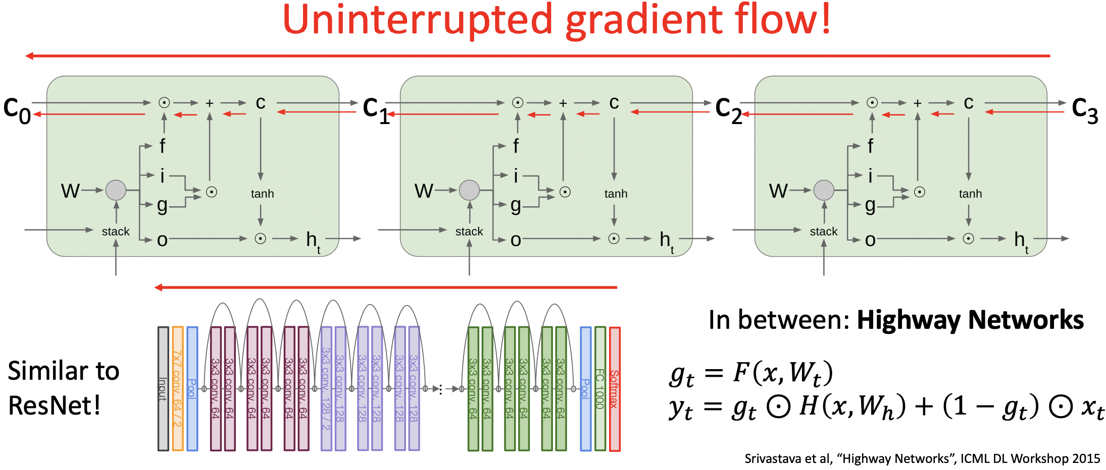
- 이 형태는 ResNet과 동일한 구조로 짜여져 있다.(skip connection)
Other RNN Variants
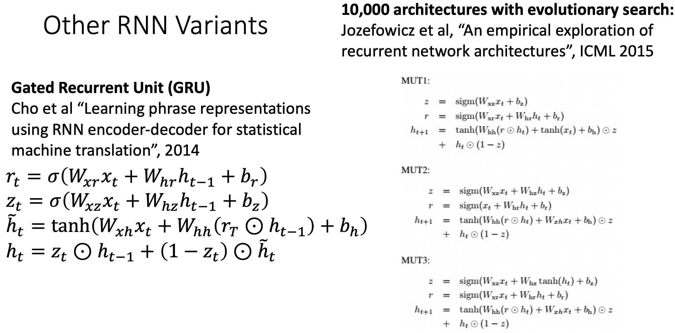
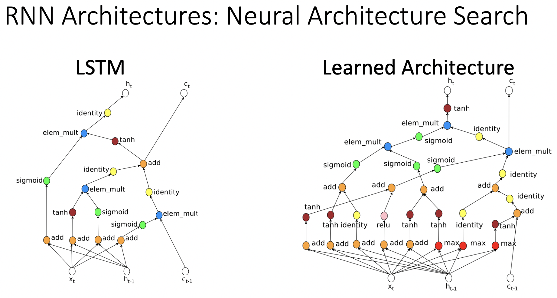
- LSTM의 연산량을 줄인 GRU와 RNN 아키텍쳐 공식을 찾는 방식도 있다.
Summary
- RNNs allow a lot of flexibility in architecture design
- Vanilla RNNs are simple but don’t work very well
- Common to use LSTM or GRU: additive interactions improve gradient flow
- Backward flow of gradients in RNN can explode or vanish.
- Exploding is controlled with gradient clipping.
- Vanishing is controlled with additive interactions (LSTM)
- Better/simpler architectures are a hot topic of current research
- Better understanding (both theoretical and empirical) is needed
참고자료
cs231n 강의 자료
cs231n 한글 강의 자료
EECS 498-007 / 598-005 2019 강의 자료
singular value
