Classification and Regression Using Supervised Learning

1 What is the difference between supervised and unsupervised learning?

지도 학습은 레이블이 달린 데이터로 학습 모델을 만들다.
비지도 학습은 레이블이 달리지 않은 데이터로 학습 모델을 만든다.

2 What is classification?

분류란, 데이터를 지정한 수만큼의 클래스로 나누는 기법이다.

샘플의 수는 다양한 상황을 반영할 수 있을 정돋로 충분해야 한다. 샘플이 부족하면 알고리즘이 학습 데이터에 필요 이상으로 최적화되는 오버피팅 현상이 발생한다.

3 How to preprocess data using various methods

현실 세계에서 추출한 방대한 양의 미가공 데이터를 다룰 때는 이를 머신 러닝 알고리즘에 학습시키기 전에 먼저 처리할 수 있는 형태로 변환하는 전처리 작업을 거쳐야 한다.

패키지 임포트

import numpy as np 
from sklearn import preprocessing

샘플데이터 정의

input_data = np.array([[5.1, -2.9, 3.3],
[-1.2, 7.8, -6.1],
[3.9, 0.4, 2.1],
[7.3, -9.9, -4.5]])

• 이진화
  : 이진화란, 숫자를 이진수로 변환하는 기법이다.

# Binarize data
data_binarized = preprocessing.Binarizer(threshold = 2.1).transform(input_data)

• 평균 제거
  : 평균 제거 기법은 특징 벡터의 값들이 0을 중심으로 분포하게 만들 때 많이 활용한다. 데이터의 값을 평균값 0, 표준편차 1로 조정하는 기법이다.

# Remove mean
data_scaled = preprocessing.scale(input_data)

• 크기 조정
  : 특징 벡터의 각 요소들을 동일 선상에서 비교할 수 있도록 값의 범위를 일정한 기준으로 조정하는 작업이다.

# Min Max scaling
data_scaler_minmax = preprocessing.MinMaxScaler(feature_range=(0,1))
data_scaled_minmax = data_scaler_minmax.fit_transform(input_data)

• 정규화
  : 특징 벡터의 값을 일정한 기준으로 측정하기 위해서는 정규화 과정을 거쳐야 한다. 대표적으로는 총 합이 1이 되도록 조정하는데 이때 각 행의 절댓값의 합이 1이 되도록 조정하는 것을 L1 정규화, 제곱의 합이 1이 되도록 조정하는 것을 L2 정규화라고 한다. 일반적으로는 이상치의 영향을 덜 받는 L1 정규화가 좀 더 안정적이다.

# Normalize data
data_normalized_l1 = preprocessing.normalize(input_data, norm='l1')
data_normalized_l2 = preprocessing.normalize(input_data, norm='l2')

4 What is label encoding?

레이블은 문자나 숫자뿐만 아니라 다양한 형태로 표현된다. 레이블은 대체로 사람이 읽기 좋도록 문자로 표현되는 경우가 많다. 하지만 사이킷런에서 제공하는 머신 러닝 함수는 숫자로 된 레이블만 처리한다. 문자로 된 레이블을 숫자로 변환하는 것을 레이블 인코딩이라고 한다.

패키지 임포트

import numpy as np 
from sklearn import preprocessing

샘플 레이블 정의

# Sample input labels
input_labels = ['red', 'black', 'red', 'green', 'balck', 'yellow', 'white']

레이블 인코딩

# Create label encoder and fit the labels
encoder = preprocessing.LabelEncoder() 
encoder.fit(input_labels)

# Print mapping 
print("\nLabel mapping:") 
for i, item in enumerate(encoder.classes_): 
    print(item, '-->', i) 

# Encode a set of labels using the encoder
test_labels = ['green', 'red', 'black'] 
encoded_values = encoder.transform(test_labels) 

# Decode a set of values using the encoder
encoded_values = [3, 0, 4, 1] 
decoded_list = encoder.inverse_transform(encoded_values) 

5 How to build a logistic regression classifier

로지스틱 회귀 분석이란 입력 변수와 출력 변수의 관계를 로지스틱 함수를 통해 계산된 확률로 표현하는 기법 중 하나다. 여기서 입력은 독립 변수이고 출력은 종속 변수다. 이때 로지스틱 함수는 시그모이드 곡선으로 표현한다. 로지스틱 함수는 데이터의 분포를 표현하는 직선 중 오차가 가장 적은 직선을 구하는 일반 선형 모델과 밀접한 관계가 있다. 엄밀히 말하면 로지스틱 분석이 분류 기법은 아니지만, 분류 문제를 다루는데 효과적이고 간결하기 때문에 머신러닝에서 굉장히 많이 사용한다.

패키지 임포트
Tkinter 패키지: https://docs.python.org/2/library/tkinter.html.

import numpy as np 
from sklearn import linear_model  
import matplotlib.pyplot as plt 
 
from utilities import visualize_classifier 

샘플 데이터 정의

# Define sample input data 
X = np.array([[3.1, 7.2], [4, 6.7], [2.9, 8], [5.1, 4.5], [6, 5], [5.6, 5], [3.3, 0.4], [3.9, 0.9], [2.8, 1], [0.5, 3.4], [1, 4], [0.6, 4.9]]) 
y = np.array([0, 0, 0, 1, 1, 1, 2, 2, 2, 3, 3, 3])

분류기 학습

# Create the logistic regression classifier
classifier = linear_model.LogisticRegression(solver='liblinear', C=1)

# Train the classifier
classifier.fit(X, y) 

# Visualize the performance of the classifier
visualize_classifier(classifier, X, y) 

• 실행 전 visualize_classifier를 정의하는 스크립트를 작성해야 한다.

import numpy as np 
import matplotlib.pyplot as plt

def visualize_classifier(classifier, X, y): 
    # Define the minimum and maximum values for X and Y
    # that will be used in the mesh grid
    min_x, max_x = X[:, 0].min() - 1.0, X[:, 0].max() + 1.0 
    min_y, max_y = X[:, 1].min() - 1.0, X[:, 1].max() + 1.0
    
    # Define the step size to use in plotting the mesh grid
    mesh_step_size = 0.01 
 
    # Define the mesh grid of X and Y values 
    x_vals, y_vals = np.meshgrid(np.arange(min_x, max_x, mesh_step_size), np.arange(min_y, max_y, mesh_step_size))
    
    # Run the classifier on the mesh grid 
    output = classifier.predict(np.c_[x_vals.ravel(), y_vals.ravel()]) 
 
    # Reshape the output array 
    output = output.reshape(x_vals.shape) 
    
    # Create a plot 
    plt.figure() 
 
    # Choose a color scheme for the plot 
    plt.pcolormesh(x_vals, y_vals, output, cmap=plt.cm.gray) 
 
    # Overlay the training points on the plot  
    plt.scatter(X[:, 0], X[:, 1], c=y, s=75, edgecolors='black', linewidth=1, cmap=plt.cm.Paired)
    
    # Specify the boundaries of the plot 
    plt.xlim(x_vals.min(), x_vals.max()) 
    plt.ylim(y_vals.min(), y_vals.max()) 
 
    # Specify the ticks on the X and Y axes 
    plt.xticks((np.arange(int(X[:, 0].min() - 1), int(X[:, 0].max() + 1), 1.0))) 
    plt.yticks((np.arange(int(X[:, 1].min() - 1), int(X[:, 1].max() + 1), 1.0))) 
 
    plt.show() 

6 What is Naïve Bayes classifier?

나이브 베이즈 분류 기법은 베이즈 정리를 기반으로 분류기를 만든다. 베이즈 정리는 사건이 발생할 확률을 그 사건에 관련된 여러 가지 조건을 기반으로 표현한다. '나이브'란 수식은 주어진 특징 값들이 서로 독립적이라고 가정하는 독립성 가정에서 왔다. 다시 말해 결과에 영향을 미치는 특성들 사이의 관계는 고려하지 않고 주어진 클래스 변수에 대한 개별 특징이 미치는 효과만 본다는 것이다.

패키지 임포트

import numpy as np 
import matplotlib.pyplot as plt 
from sklearn.Naïve_bayes import GaussianNB  
from sklearn import cross_validation 
 
from utilities import visualize_classifier 

input data 읽어오기

# Input file containing data 
input_file = 'data_multivar_nb.txt

# Load data from input file 
data = np.loadtxt(input_file, delimiter=',') 
X, y = data[:, :-1], data[:, -1]

분류기 학습 및 예측

# Create Naïve Bayes classifier 
classifier = GaussianNB() 

# Train the classifier 
classifier.fit(X, y)

# Predict the values for training data 
y_pred = classifier.predict(X)

분류기 성능 확인

# Compute accuracy 
accuracy = 100.0 * (y == y_pred).sum() / X.shape[0] 
print("Accuracy of Naïve Bayes classifier =", round(accuracy, 2), "%") 
 
# Visualize the performance of the classifier 
visualize_classifier(classifier, X, y) 

• 이렇게 정확도를 측정하는 방식은 완벽하지 않다. 데이터를 학습용과 테스트용으로 나누어 교차 검증 기법을 활용하는 것이 좋다.

# Split data into training and test data  
X_train, X_test, y_train, y_test = cross_validation.train_test_split(X, y, test_size=0.2, random_state=3) 
classifier_new = GaussianNB() 
classifier_new.fit(X_train, y_train) 
y_test_pred = classifier_new.predict(X_test) 

# compute accuracy of the classifier
accuracy = 100.0 * (y_test == y_test_pred).sum() / X_test.shape[0] 
print("Accuracy of the new classifier =", round(accuracy, 2), "%") 
 
# Visualize the performance of the classifier 
visualize_classifier(classifier_new, X_test, y_test) 

정확도 정밀도 재현율 계산

num_folds = 3 
accuracy_values = cross_validation.cross_val_score(classifier,  
        X, y, scoring='accuracy', cv=num_folds) 
print("Accuracy: " + str(round(100*accuracy_values.mean(), 2)) + "%") 
 
precision_values = cross_validation.cross_val_score(classifier,  
        X, y, scoring='precision_weighted', cv=num_folds) 
print("Precision: " + str(round(100*precision_values.mean(), 2)) + "%") 
 
recall_values = cross_validation.cross_val_score(classifier,  
        X, y, scoring='recall_weighted', cv=num_folds) 
print("Recall: " + str(round(100*recall_values.mean(), 2)) + "%") 
 
f1_values = cross_validation.cross_val_score(classifier,  
        X, y, scoring='f1_weighted', cv=num_folds) 
print("F1: " + str(round(100*f1_values.mean(), 2)) + "%")

7 What is a confusion matrix?

오차 행렬이란 분류기의 성능을 표현한 그림 또는 표다.

• 참 양성: 예측 결과가 1이고 GT 값도 1인 샘플
• 참 음성: 예측 결과가 1이고 GT 값도 0인 샘플
• 거짓 양성: 예측 결과가 0이고 GT 값도 0인 샘플, 1종 오류라고 부른다.
• 거짓 음성: 예측 결과가 0이고 GT 값도 1인 샘플, 2종 오류라고 부른다.

패키지 임포트

import numpy as np 
import matplotlib.pyplot as plt 
from sklearn.metrics import confusion_matrix 
from sklearn.metrics import classification_report

샘플 레이블 정의

# Define sample labels 
true_labels = [2, 0, 0, 2, 4, 4, 1, 0, 3, 3, 3] 
pred_labels = [2, 1, 0, 2, 4, 3, 1, 0, 1, 3, 3] 

오차행렬

# Create confusion matrix 
confusion_mat = confusion_matrix(true_labels, pred_labels)

# Visualize confusion matrix 
plt.imshow(confusion_mat, interpolation='nearest', cmap=plt.cm.gray) 
plt.title('Confusion matrix') 
plt.colorbar() 
ticks = np.arange(5) 
plt.xticks(ticks, ticks) 
plt.yticks(ticks, ticks) 
plt.ylabel('True labels') 
plt.xlabel('Predicted labels') 
plt.show()

분류기 성능 출력

# Classification report 
targets = ['Class-0', 'Class-1', 'Class-2', 'Class-3', 'Class-4'] 
print('\n', classification_report(true_labels, pred_labels, target_names=targets)) 

8 What are Support Vector Machines and how to build a classifier based on that?

서포트 벡터 머신은 클래스를 구분하는 경계선을 직선이 아닌 초평면으로 표현한다. 여기서 초평면이란 쉽게 말해 직선을 N차원으로 표현한 것이다.

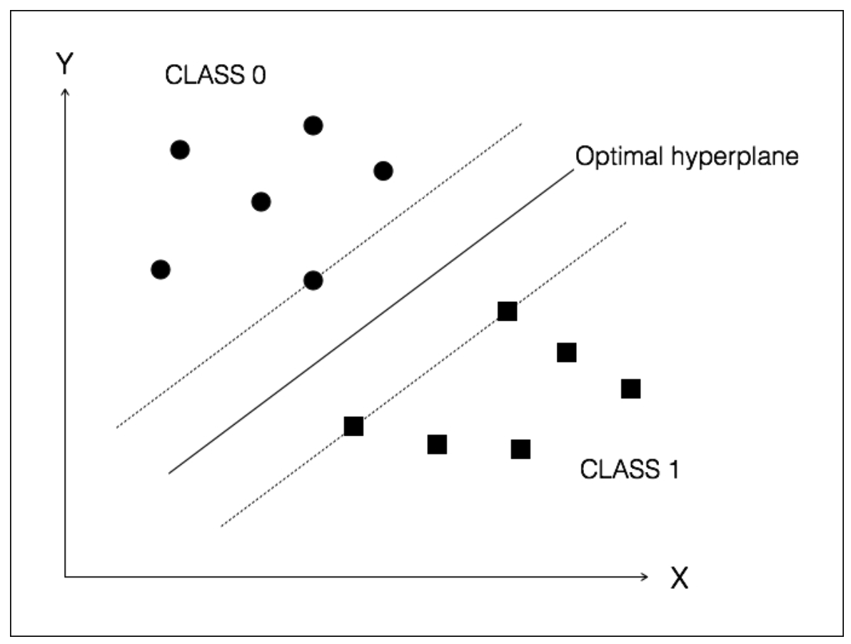
위는 주어진 데이터를 두개의 class로 분류한 초평면이다. 그림 속 실선은 두 클래스의 점들 사이의 거리를 최대화한 최적의 초평면이고 점선은 서포트 벡터이다. 서포트 벡터 사이의 거리를 최대 마진이라고 한다.

패키지 임포트

import numpy as np 
import matplotlib.pyplot as plt 
from sklearn import preprocessing 
from sklearn.svm import LinearSVC 
from sklearn.multiclass import OneVsOneClassifier 
from sklearn import cross_validation

데이터 로드

# Input file containing data 
input_file = 'income_data.txt

# Read the data 
X = [] 
y = [] 
count_class1 = 0 
count_class2 = 0 
max_datapoints = 25000 

with open(input_file, 'r') as f: 
    for line in f.readlines(): 
        if count_class1 >= max_datapoints and count_class2 >= max_datapoints: 
            break 
 
        if '?' in line: 
            continue
            ‘data = line[:-1].split(', ') 
 
        if data[-1] == '<=50K' and count_class1 < max_datapoints: 
            X.append(data) 
            count_class1 += 1 
 
        if data[-1] == '>50K' and count_class2 < max_datapoints: 
            X.append(data) 
            count_class2 += 1
            
# Convert to numpy array 
X = np.array(X)

# Convert string data to numerical data 
label_encoder = []  
X_encoded = np.empty(X.shape) 
for i,item in enumerate(X[0]): 
    if item.isdigit():  
        X_encoded[:, i] = X[:, i] 
    else: 
        label_encoder.append(preprocessing.LabelEncoder()) 
        X_encoded[:, i] = label_encoder[-1].fit_transform(X[:, i]) 
 
X = X_encoded[:, :-1].astype(int) 
y = X_encoded[:, -1].astype(int)

SVM 모델 학습

# Create SVM classifier 
classifier = OneVsOneClassifier(LinearSVC(random_state=0))

# Train the classifier 
classifier.fit(X, y)

모델 성능 확인

# Cross validation 
X_train, X_test, y_train, y_test = cross_validation.train_test_split(X, y, test_size=0.2, random_state=5) 
classifier = OneVsOneClassifier(LinearSVC(random_state=0)) 
classifier.fit(X_train, y_train) 
y_test_pred = classifier.predict(X_test)

# Compute the F1 score of the SVM classifier 
f1 = cross_validation.cross_val_score(classifier, X, y, scoring='f1_weighted', cv=3) 
print("F1 score: " + str(round(100*f1.mean(), 2)) + "%")

# Predict output for a test datapoint 
input_data = ['37', 'Private', '215646', 'HS-grad', '9', 'Never-married', 'Handlers-cleaners', 'Not-in-family', 'White', 'Male', '0', '0', '40', 'United-States']

# Encode test datapoint
input_data_encoded = [-1] * len(input_data) 
count = 0 
for i, item in enumerate(input_data): 
    if item.isdigit(): 
        input_data_encoded[i] = int(input_data[i]) 
    else: 
        input_data_encoded[i] = int(label_encoder[count].transform(input_data[i])) 
        count += 1  
 
input_data_encoded = np.array(input_data_encoded)

# Run classifier on encoded datapoint and print output 
predicted_class = classifier.predict(input_data_encoded) 
print(label_encoder[-1].inverse_transform(predicted_class)[0]) 

9 What is linear and polynomial regression?

회귀 분석이란 입력 변수와 출력 변수의 관계를 추정하는 기법이다. 이때 입력 변수끼리는 서로 독립적이지 않아도 된다. 입력 변수 사이에 상관관계가 있는 경우가 비일비재하기 때문이다

회귀 분석 기법 중 선형 회귀 분석은 입력과 출력의 관계가 선형이라고 가정한다. 모델링 관점에서 보면 제약이 심하지만 속도가 빠르고 효과적이다.

다항 회귀 분석은 선형 회귀 분석만으로 밝혀내기 힘든 관계를 추출할 때 확용한다. 선형 회귀보다 계산이 복잡하지만 정확도가 높다.

10 How to build a linear regressor for single variable and multivariable data

1 선형 회귀 분석

import pickle 
 
import numpy as np 
from sklearn import linear_model 
import sklearn.metrics as sm 
import matplotlib.pyplot as plt

# Input file containing data 
input_file = 'data_singlevar_regr.txt'

# Read data 
data = np.loadtxt(input_file, delimiter=',') 
X, y = data[:, :-1], data[:, -1]

# Train and test split 
num_training = int(0.8 * len(X)) 
num_test = len(X) - num_training 
 
# Training data 
X_train, y_train = X[:num_training], y[:num_training] 
 
# Test data 
X_test, y_test = X[num_training:], y[num_training:]

# Create linear regressor object 
regressor = linear_model.LinearRegression() 
 
# Train the model using the training sets 
regressor.fit(X_train, y_train)

# Predict the output 
y_test_pred = regressor.predict(X_test)

# Plot outputs 
plt.scatter(X_test, y_test, color='green') 
plt.plot(X_test, y_test_pred, color='black', linewidth=4) 
plt.xticks(()) 
plt.yticks(()) 
plt.show() 

# Compute performance metrics 
print("Linear regressor performance:") 
print("Mean absolute error =", round(sm.mean_absolute_error(y_test, y_test_pred), 2)) 
print("Mean squared error =", round(sm.mean_squared_error(y_test, y_test_pred), 2))  
print("Median absolute error =", round(sm.median_absolute_error(y_test, y_test_pred), 2))  
print("Explain variance score =", round(sm.explained_variance_score(y_test, y_test_pred), 2)) 
print("R2 score =", round(sm.r2_score(y_test, y_test_pred), 2)) 

# Model persistence 
output_model_file = 'model.pkl' 
 
# Save the model 
with open(output_model_file, 'wb') as f: 
    pickle.dump(regressor, f)
    
# Load the model 
with open(output_model_file, 'rb') as f: 
    regressor_model = pickle.load(f)
    
# Perform prediction on test data 
y_test_pred_new = regressor_model.predict(X_test) 
print("\nNew mean absolute error =", round(sm.mean_absolute_error(y_test, y_test_pred_new), 2))

2 다항 회귀 분석

import numpy as np 
from sklearn import linear_model 
import sklearn.metrics as sm 
from sklearn.preprocessing import PolynomialFeatures

# Input file containing data 
input_file = 'data_multivar_regr.txt'

# Load the data from the input file 
data = np.loadtxt(input_file, delimiter=',') 
X, y = data[:, :-1], data[:, -1]

# Split data into training and testing  
num_training = int(0.8 * len(X)) 
num_test = len(X) - num_training 
 
# Training data 
X_train, y_train = X[:num_training], y[:num_training] 
 
# Test data 
X_test, y_test = X[num_training:], y[num_training:] 

# Create the linear regressor model 
linear_regressor = linear_model.LinearRegression() 
 
# Train the model using the training sets 
linear_regressor.fit(X_train, y_train) 

# Predict the output 
y_test_pred = linear_regressor.predict(X_test)

# Measure performance 
print("Linear Regressor performance:") 
print("Mean absolute error =", round(sm.mean_absolute_error(y_test, y_test_pred), 2)) 
print("Mean squared error =", round(sm.mean_squared_error(y_test, y_test_pred), 2)) 
print("Median absolute error =", round(sm.median_absolute_error(y_test, y_test_pred), 2)) 
print("Explained variance score =", round(sm.explained_variance_score(y_test, y_test_pred), 2)) 
print("R2 score =", round(sm.r2_score(y_test, y_test_pred), 2)) 

# Polynomial regression 
polynomial = PolynomialFeatures(degree=10) 
X_train_transformed = polynomial.fit_transform(X_train) 
datapoint = [[7.75, 6.35, 5.56]] 
poly_datapoint = polynomial.fit_transform(datapoint) 

poly_linear_model = linear_model.LinearRegression() 
poly_linear_model.fit(X_train_transformed, y_train) 
print("\nLinear regression:\n", linear_regressor.predict(datapoint)) 
print("\nPolynomial regression:\n", poly_linear_model.predict(poly_datapoint)) 

11 How to estimate housing prices using Support Vector Regressor

실습 코드

import numpy as np 
from sklearn import datasets 
from sklearn.svm import SVR 
from sklearn.metrics import mean_squared_error, explained_variance_score 
from sklearn.utils import shuffle 

# Load housing data 
data = datasets.load_boston()

# Shuffle the data 
X, y = shuffle(data.data, data.target, random_state=7)

# Split the data into training and testing datasets  
num_training = int(0.8 * len(X)) 
X_train, y_train = X[:num_training], y[:num_training] 
X_test, y_test = X[num_training:], y[num_training:]

# Create Support Vector Regression model 
sv_regressor = SVR(kernel='linear', C=1.0, epsilon=0.1)

# Train Support Vector Regressor 
sv_regressor.fit(X_train, y_train) 

# Evaluate performance of Support Vector Regressor 
y_test_pred = sv_regressor.predict(X_test) 
mse = mean_squared_error(y_test, y_test_pred) 
evs = explained_variance_score(y_test, y_test_pred)  
print("\n#### Performance ####") 
print("Mean squared error =", round(mse, 2)) 
print("Explained variance score =", round(evs, 2))

# Test the regressor on test datapoint 
test_data = [3.7, 0, 18.4, 1, 0.87, 5.95, 91, 2.5052, 26, 666, 20.2, 351.34, 15.27] 
print("\nPredicted price:", sv_regressor.predict([test_data])[0])