---

Cross Validation

1. K-fold

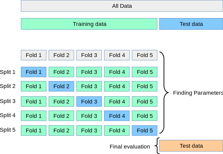
k-fold는 데이터를 k개로 쪼개는것을 말한다.
일반적으로 Cross Validation에서 사용하고 k-1개의 모델에서 학습하고 1개의 테스트 모델에서 검증한다.
-> k번의 다른 데이터셋으로 학습이 가능하다는 장점

k-fold 대표 파라미터

• n_splits (int) : Fold의 개수 k 값
• shuffle (bool) : 데이터를 쪼갤 때 섞을지 유무
• random_state (int) : 내부적으로 사용되는 난수값

실습

from sklearn.model_selection import KFold
kf = KFold(n_splits=5, shuffle=True, random_state=42)

for i, (trn_idx, val_idx) in enumerate(kf.split(data, label)):
    x_train, y_train = data.iloc[trn_idx, :], label[trn_idx,]
    x_valid, y_valid = data.iloc[val_idx, :], label[val_idx,]

    print('{} Fold, trn label\n Open: {}, Close: {}'.format(i,   np.sum(y_train == 1), np.sum(y_train == 0)))
    print('{} Fold, val label\n Open: {}, Close: {}\n'.format(i, np.sum(y_valid == 1), np.sum(y_valid == 0)))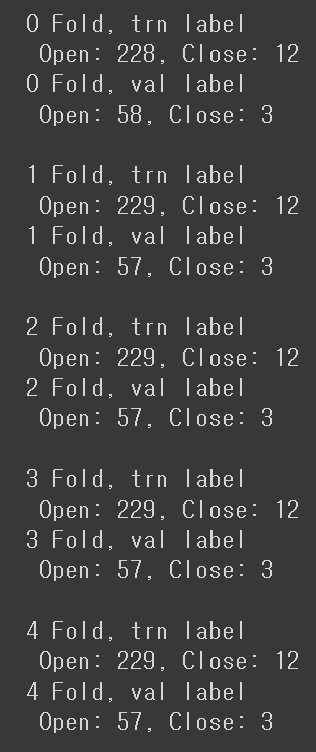

2. Strartified K-fold

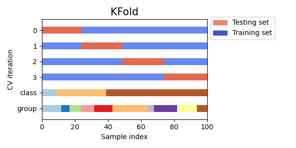
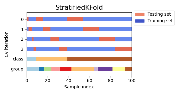
k-fold 에서 fold를 할때 한 클래스의 분포가 너무 많거나, 적게 나올 수가 있어서 이 문제를 해결하기 위해 나온 방식.
데이터셋의 클래스의 비율을 맞춰서 쪼개준다.

Strartified K-fold 대표 파라미터

• n_splits (int) : Fold의 개수 k 값
• shuffle (bool) : 데이터를 쪼갤 때 섞을지 유무
• random_state (int) : 내부적으로 사용되는 난수값

실습

from sklearn.model_selection import StratifiedKFold
skf = StratifiedKFold(n_splits=5, shuffle=True, random_state=42)

for i, (trn_idx, val_idx) in enumerate(skf.split(data, label)):
    x_train, y_train = data.iloc[trn_idx, :], label[trn_idx,]
    x_valid, y_valid = data.iloc[val_idx, :], label[val_idx,]

    print('{} Fold, trn label\n Open: {}, Close: {}'.format(i,   np.sum(y_train == 1), np.sum(y_train == 0)))
    print('{} Fold, val label\n Open: {}, Close: {}\n'.format(i, np.sum(y_valid == 1), np.sum(y_valid == 0)))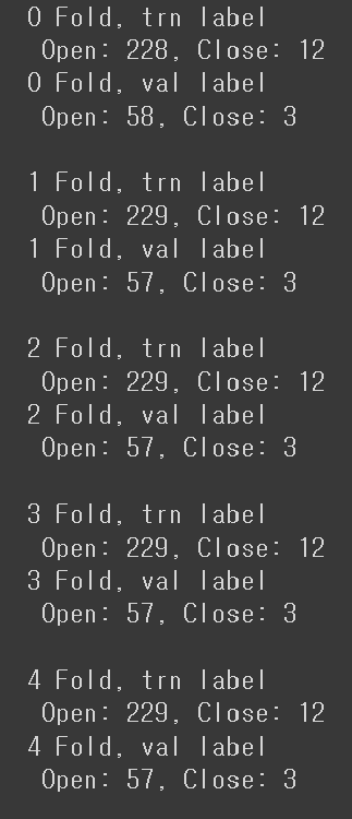

Stratified K-fold 를 이용한 Cross Validation

from sklearn.ensemble import RandomForestClassifier
from sklearn.metrics  import f1_score

val_scores = list()

skf = StratifiedKFold(n_splits=5, shuffle=True, random_state=42)

for i, (trn_idx, val_idx) in enumerate(skf.split(data, label)):
  x_train, y_train = data.iloc[trn_idx], label[trn_idx]
  x_valid, y_valid = data.iloc[val_idx], label[val_idx]

  # 전처리
  x_train, x_valid, x_test = preprocess(x_train, x_valid, test)


  # 모델 정의
  model = RandomForestClassifier()

  # 모델 학습
  model.fit(x_train, y_train)

  # 훈련, 검증 데이터 f1_score 확인
  trn_f1 = f1_score(y_train, model.predict(x_train))
  val_f1 = f1_score(y_valid, model.predict(x_valid))
  print('{} Fold, train f1_score : {:.4f}4, validation f1_score : {:.4f}'.format(i, trn_f1, val_f1))

  val_scores.append(val_f1)

# 교차 검증 f1_score 평균 계산하기
print('Cross Validation Score : {:.4f}'.format(np.mean(val_scores)))

---

Ensemble

여러 모델을 학습시켜서 좋은 모델 찾는 방법

1. Voting Ensemble

각자의 모델이 투표를 하여 클래스를 선택하는 방식의 앙상블

Hard, Soft로 Voting 방식이 나뉘는데, Hard는 라벨 값으로 투표를 하는 방식이고, Soft는 확률 값을 모두 더해 가장 높은 클래스를 선택합니다.

Voting Classifier는 Sklearn의 ensemble 패키지에 있습니다.

실습

from sklearn.ensemble import VotingClassifier
from sklearn.linear_model import LogisticRegression
from sklearn.neural_network import MLPClassifier

clfs = [['Logistic', LogisticRegression()],
      ['RandomForest', RandomForestClassifier()],
      ['MLP', MLPClassifier()]]

vote_clf = VotingClassifier(clfs, voting='soft', n_jobs=4)

# 여기서 x_train, y_train은 마지막 Fold
vote_clf.fit(x_train, y_train)

print('Validation F1 score : {:.4f}'.format(f1_score(y_valid, vote_clf.predict(x_valid))))

voting hard는 predict_proba 메소드가 지원이 되지 않는다.
vote_clf.predict_proba(x_valid)

2. Out-of-fold(OOF) Ensemble

OOF 앙상블은 KFold 교차 검증에서 생성되는 각 Fold에 대한 예측 값을 앙상블하는 기법으로 모델 검증과 함께 앙상블을 진행할 수 있다는 장점이 있습니다.

  val_scores = list()
oof_pred = np.zeros((test.shape[0], le.classes_.shape[0]))

skf = StratifiedKFold(n_splits=5, shuffle=True, random_state=42)

for i, (trn_idx, val_idx) in enumerate(skf.split(data, label)):
    x_train, y_train = data.iloc[trn_idx], label[trn_idx]
    x_valid, y_valid = data.iloc[val_idx], label[val_idx]

    # 전처리
    x_train, x_valid, x_test = preprocess(x_train, x_valid, test)


    # 모델 정의
    clf = RandomForestClassifier()

    # 모델 학습
    clf.fit(x_train, y_train)

    # 훈련, 검증 데이터 f1_score 확인
    trn_f1 = f1_score(y_train, clf.predict(x_train))
    val_f1 = f1_score(y_valid, clf.predict(x_valid))
    print('{} Fold, train f1_score : {:.4f}4, validation f1_score : {:.4f}'.format(i, trn_f1, val_f1))

    val_scores.append(val_f1)

    # 결과 모으기
    oof_pred += clf.predict_proba(x_test) / skf.n_splits

# 교차 검증 f1_score 평균 계산하기
print('Cross Validation Score : {:.4f}'.format(np.mean(val_scores)))

np.argmax(oof_pred, axis=1) # 각 라벨별로 어떻게 예측했는지 argmax로 확인가능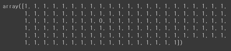

Feature Selection

Permutation Importance

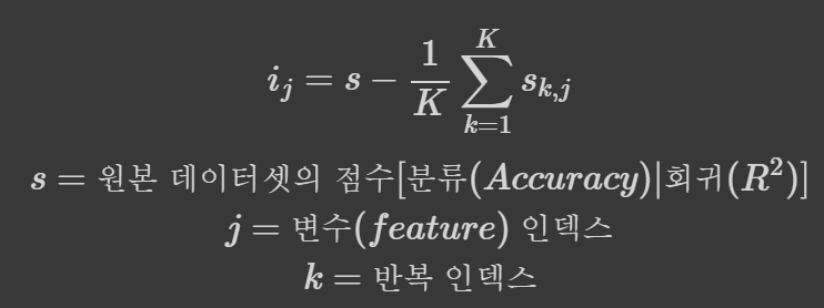
Permutation Importance의 기본 원리는 어떤 변수를 임의로 섞어 그 중 타겟 변수에 영향을 많이 주는 변수를 탐색합니다.
예를 들어 타겟 변수를 예측하기 좋은 변수는 임의로 섞었을 경우 모델의 성능이 많이 떨어지게되는데, 이러한 방식으로 좋은 변수를 선별해 냅니다.

실습

from sklearn.ensemble import RandomForestClassifier
from sklearn.inspection import permutation_importance

model = RandomForestClassifier(random_state=42, n_jobs=-1)
model.fit(x_train, y_train)

r = permutation_importance(model, x_valid, y_valid,
                         n_repeats=10,
                         random_state=42,
                         scoring='neg_log_loss')

for i in r.importances_mean.argsort()[::-1]:
  if r.importances_mean[i] - 2 * r.importances_std[i] > 0:
# 이 조건식은 이상치를 제외하고 어느정도 평균 근처값만 보기위함인듯
      print(f"{x_valid.columns[i]:<8}: "
             f"{r.importances_mean[i]:.3f}"
             f" +/- {r.importances_std[i]:.3f}")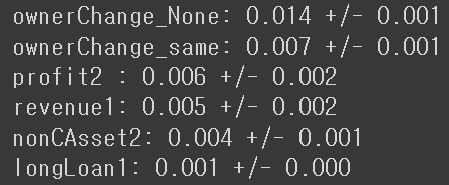

AutoML

Optuna

데이터의 형태 혹은 도메인에 따라 성능이 좋거나, 괜찮다고 알려진 모델들은 많습니다. 하지만 해당 모델들의 기본 설정 값을 이용한다면 우리 데이터에 좋은 성능을 낼 수 있을까요? 대부분 그렇지 않습니다. 따라서 우리 데이터에 좋은 성능을 낼 수 있도록 모델 파라미터를 조정해주어야합니다. 이를 Hyter Parameter Tuning, HPO 라 합니다.

많이 알려진 라이브러리로 Optuna, HypterOpt, Scikit-Opt 등이 있지만, Optuna가 좀 더 직관적이고 사용하기 쉽습니다.

주요 특징

• 가볍고 다양한 플랫폼에 구애 받지 않는 구조
• 조건 및 루프를 통한 손쉬운 Search Space 정의
• 효율적인 최적화 알고리즘
• 쉬운 병렬화
• 빠른 시각화
  

1. objective function

먼저 최적화 할 대상 함수인 objective 함수를 작성해야 합니다.
학습 로직 및 튜닝할 파라미터의 목록을 작성합니다.
Optuna에서 지원하는 Search Space 함수는 범주형, 실수형, 정수형, 이산 균등분포, 균등, 로그 균등 분포 등이 있습니다.
-> Optuna search space 함수 리스트

objective 함수의 반환 값은 우리가 튜닝하고자 하는 메트릭을 반환하면 됩니다.

!pip install optuna

import optuna
from xgboost import XGBClassifier
from sklearn.metrics import roc_auc_score

def objective(trial):
    # 튜닝할 파라미터 목록
    n_estimators = trial.suggest_int('n_estimators', 100, 500)
    max_depth = trial.suggest_int('max_depth', 1, 10)
    subsample = trial.suggest_float('subsample', 0.5, 1.0)
    colsample_bytree = trial.suggest_float('colsample_bytree', 0.5, 1.0)

    # Ensemble 실습에서 사용한 마지막 데이터셋
    x_train, y_train = data.iloc[trn_idx], label[trn_idx]
    x_valid, y_valid = data.iloc[val_idx], label[val_idx]

    # 데이터 전처리
    x_train, x_valid, x_test = preprocess(x_train, x_valid, test)

    # 모델 정의
    model = XGBClassifier(n_estimators=n_estimators,
                          max_depth=max_depth,
                          subsample=subsample,
                          colsample_bytree=colsample_bytree,
                          random_state=42)

    # 모델 학습
    model.fit(x_train, y_train,
              eval_metric='auc',
              eval_set=[[x_train, y_train], [x_valid, y_valid]],
              early_stopping_rounds=30,
              verbose=None)

    # 검증 데이터 메트릭
    val_auc = roc_auc_score(y_valid, model.predict_proba(x_valid)[:, 1])

    # 튜닝할 메트릭
    return val_auc

2. Study 정의 및 튜닝 시작하기

objective 함수가 준비 되었다면, Optuna Study 객체를 생성 후 튜닝을 시작할 수 있습니다.
study 객체 생성 시, 튜닝할 방향을 설정할 수 있습니다.
study.optimize 메소드로 튜닝을 시작하며, objective 함수와 튜닝 횟수를 전달하면 됩니다.

# study 생성
study = optuna.create_study(direction="maximize") # or minimize

study.optimize(objective, n_trials=100, )

3. Best Parameter

파라미터 튜닝이 끝났다면, study 객체에서 가장 좋은 성능을 냈던 파라미터와 메트릭을 확인할 수 있습니다.

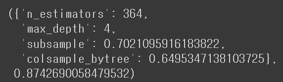
study.best_params, study.best_value