일요일 오전, 또 유행병에 내 일상이 강타당했다.
잔잔히 시간을 한번씩 보내고 오며, 작은 용돈벌이를 하는 카페의 저녁 직원의 감염.
지난 주에 자가격리가 해제돼서 근무했는데, KF94 쓰면서 음식도 안 먹으려다가
분명 본인은 안 걸린다며 조금 멀찍이 각자 식사를 했는데 결국 감염되셨다 ㅠㅠ...
나로 인한 전염인지, 다른데서 온 전염인지는 모르겠지만
갑작스럽게 저녁 알바를 하게 되었는데
안그래도 요즘 건강때문에 생활 패턴 정상화를 해야 했어서
아침일찍 일어나 미선이와 카페에서 스터디 :) 밤까지 카페일하고 집가서 쭉 자야지.
다행히 오늘까지 제출인 과제도 다 넉넉하게 마무리해뒀던 터라, 여유있게 강의내용 복습을 위해 카페 오픈 전, 근처 다른 카페에서 공부를 해본다.

Review of Lecture 1 - 3

(1) Defining a Classifier

s = f(x;W) = Wx  

function f
parameterized by weights W
taking data x as input
vector of scores s as output for each of the classes (in classification)

(2) Loss Function (SVM)

Loss function : quantifies how happy / unhappy we are with the scores (output)

Li = Sigma ~~. 이거 다시 적기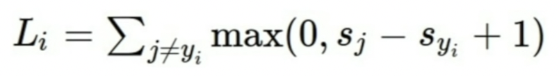

combination of data term L
regularization term that expresses how simple out model is (preference for simpler models for better generization)
parameters

we want parameters w - that correspond to lowest loss (minimizing loss function)

for this, we must find gradient L with respect to W :

여기서 with respect to W 는 대충 W에 관한 L의 기울기니까,
대충 x,y축 그래프로 생각하면 x축으로 다양한 w 값이 있을 때, 그에 대한 y축 L의 최솟값을 찾는 것.
어려운 개념은 아니지만 영어로 생각하려더니 조금 헷갈림 한번씩.

(3) Optimization

iteratively taking steps in direction of steepest descent (negative of gradient) ,
to find the point with lowest loss.

왜 -gradient 가 lowest loss 지? 감소폯을 얘기하는건가

gradient! 이 particular element가 final output 에 얼마나 영향을 미치는 지 나타내준다 볼 수 있음.

Gradient descent

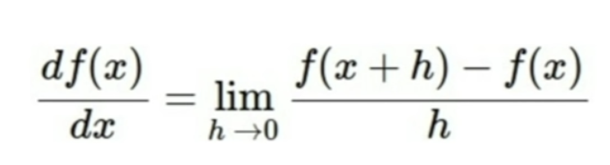
Numerical Gradient : slow, approximate, easy to write
Analytic Gradient : fast, exact, error-prone :(

In practice -> Derive analytic gradient, check your implementation with numerical gradient

각각의 장단점을 고려해 보완하는 방향으로!

---

Lecture 4 - Back Propogation & Neural Networks

(1) Back Propogation

1. Computational Graph

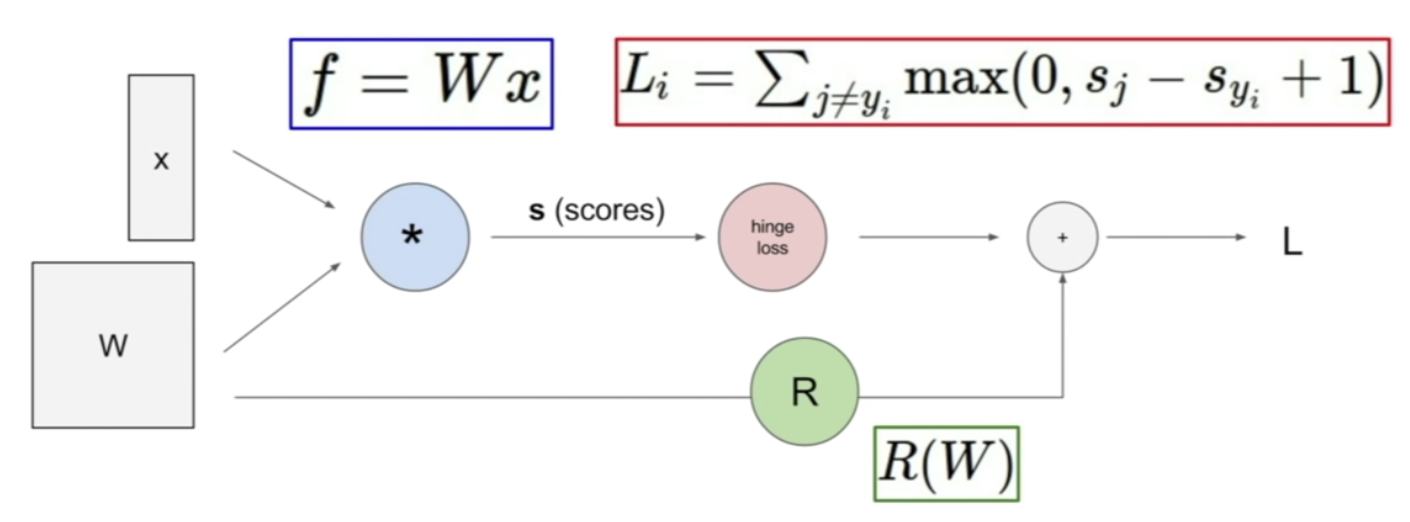
Using a graph to represent any function, as nodes - steps of functions we go through

• : f=Wx
  hinge loss : computing data loss Li
  Regularization : R(W)
  L : sum of regularization term & data term

with this, back propogation is possible!

2. Back Propogation

revursively using the chain rule in order to compute the gradient with respect to every variable in the computational graph

input has to go through many transitions through deep learning models to

how it works - example (1)

represent function f with a computational graph

first node : x + y
second node : (firt node's output / intermediate value : x+y)*z

given the values of the variables, computational graph

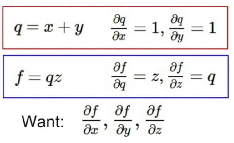
give every intermediate variable a name
q : intermediate variable after the plus node = x+y
f = qz

q 우편에는 gradient of q with respect to x and y
f 우편에는 gradient of f with respect to z and q

what we want - gradients of f (the entire computation) / x, y, z

Backprop - recursive application of chain rule

start from the back, compute all the gradients along the way backwards.

second node backprop : df/dz = q, df/dq = z
first node backprop : dq/dx = 1, dq/dy = 1

df/dq = -4

df/dy = ?
y is not connected directly to f.

to find the effect of y on f,
we leverage the chain rule.
df/dy = df/dq dq/dy = df/dq 1 = z * 1 = z

• what we can notice? the change of y - effect on q will be 1 (same) - effect on f will be -4!
  df/dy = -4

df/dx = ?
same procedure -
df/dx = df/dq dq/dx = df/dq 1 = z * 1 = z
df/dx = -4

basic idea of back propagation

each node is only aware of its immediate surrounding at initial state

• local inputs connected to nodes and direct output from node
• from this, "local gradient" are found.

방금 예시에서 intermediate value q of first node가 x, y, 그리고 second node 와만 직접적으로 연결되어 있었듯이,
그래서 gradient dq/dx, dq/dy가 local graident
...
그냥 미분하는 것이셈 ~ 물론... 나중에 공식들이 복잡해지면 직접 미분으로는 해결이 어려우니까 컴을 써야겠지

during back prop - at each node we have the upstream gradients coming back.

how df/dq was done first, and passed back

gradient of Final loss L, with respect to just before the node is calculated at every node's direct back propogation

계속 뒤로 곱하게 되는 것이셈~~ chain rule 땜에 so EZ

how it works - example (2)

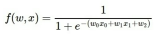
1. write out as computational graph

2. make forward pass, and make up the values of at every stage of computation

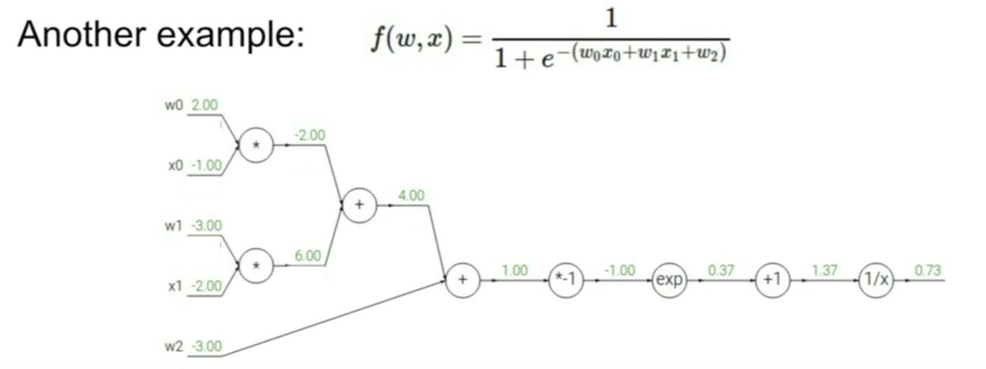
3. backward propogate using calculus & chain rule

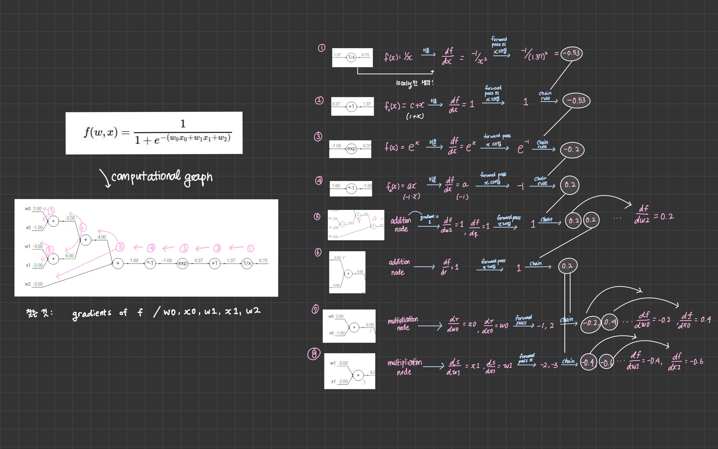
3. Patterns in Backward Flow

1. add gate : gradient distributor - takes the upstream gradient and passes it on .
   ex) addition node

2. max gate : gradient router - one takes the full value of gradient just passed back (1) , the other takes gradient of zero (0)

   why?

   In forward pass, only the maximum value gets passed down to rest of computation and thus affecting the function computation -

   In passing back, we want to adjust back propogation, to flow it through that same branch of computation

3. mul gate : gradient switcher - takes upstream gradient and switch/scale it by the value of the other branch

   local gradient is just the value of the other variable

4. Back Propogation and Optimization

By being able to compute gradients,
we can apply it in optimization to update our parameters (weights, biases ... ) !

df/dx = sum of df/dq*dq/dx (q being intermediate nodes local output values)

5. Back Propogation with Vectors

everything is same - except, the gradients will be Jacobian Matrices

how it works - example (1)

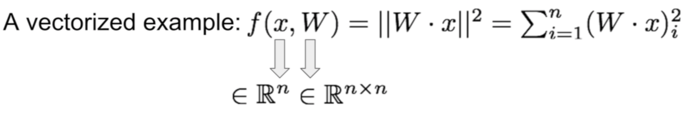
x : n-dimensional
W : n * n

1. Computational Graph

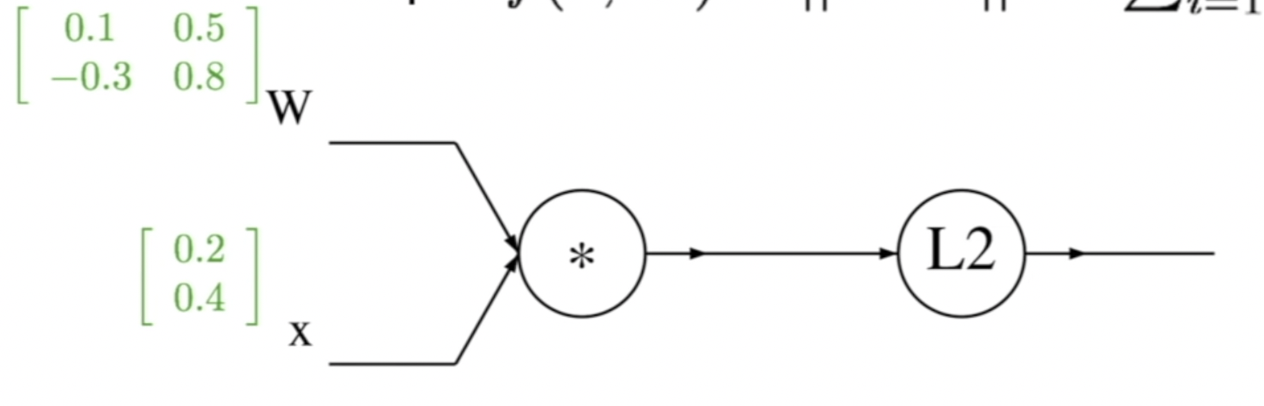
2. q = intermediate value after first node ()
   

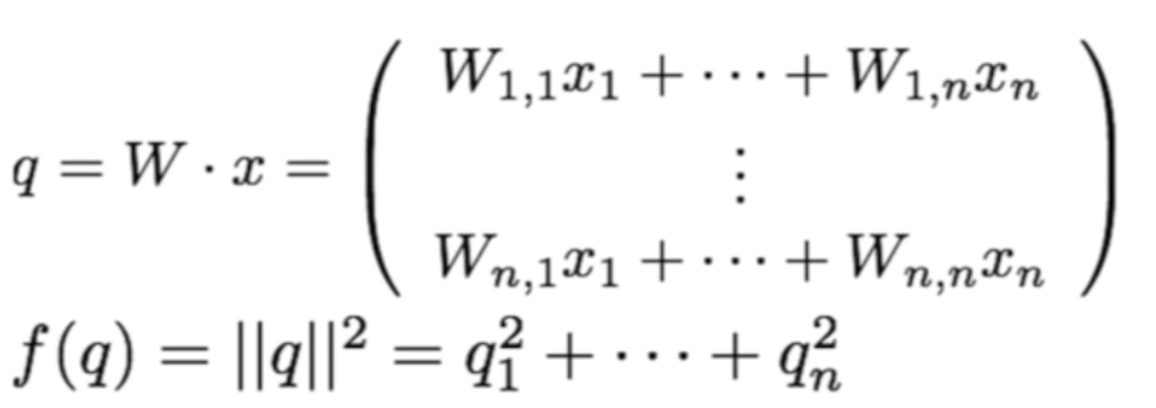
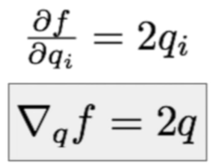
3. backprop - calculus & local derivative

(1) intermediate node - derivative of f with respect to qi

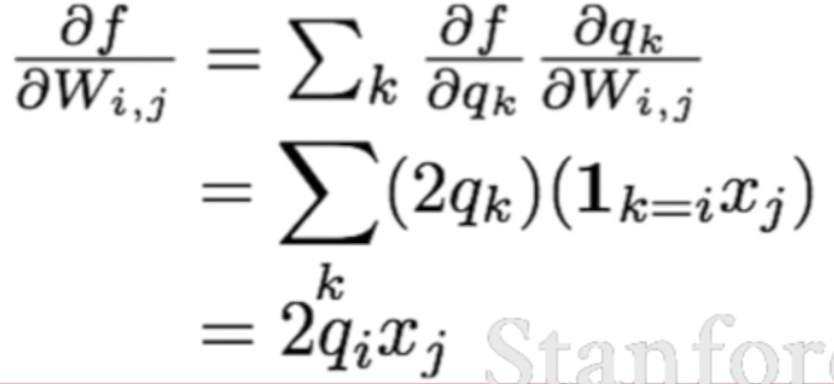
(2) W - derivative of qk with respect to W

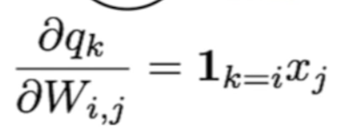
chain rule! derivative of f with respect to W

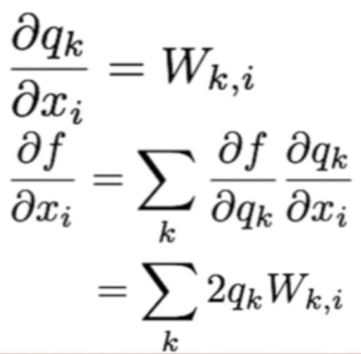
(3) x - derivative of q with respect to xi,
chain rule! derivative of f with respect to xi

6. Modularized Implementation

implement forward pass,
cache the values

implement backward pass

(2) Neural Networks

1. 2-layer Neural Network

Linear Score Function (여태깔짝대던거)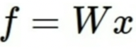

multiple-layer Neural Network -

• 2-layer NN
  

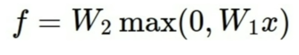
  a neural network - with a form of 2 linear score functions stacked together

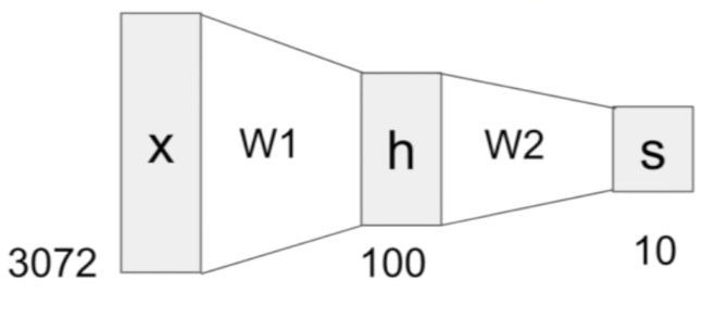
• input - matrix 1 = x*W1, linear
• first layer - (matrix 1 = x* W1, value of scores h) non-linearity implemented directly before h
• h - max(x*W1)
• second layer - (h, s) ex/max of zero
• output - score function, linear

Classifying Horses Example
W1 - high score for left-facing horses ?
W2 -
...뭐라는거임 설명

• 3-layer NN
  

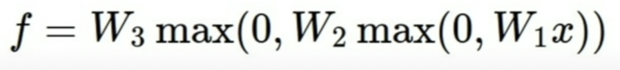
like this... deep NNs can be made ~ yay

2. Biological Inspiration of Deep NNs - Neurons

neuron

neurons connected together

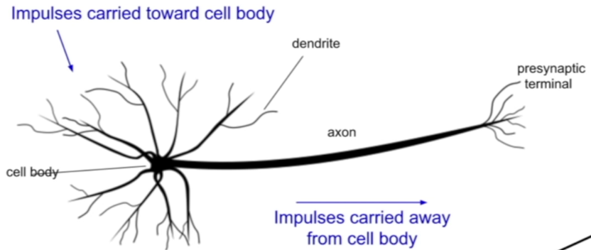
Dendrites : Impulses are received (inputs)
Cell Body : Integrates Impulses/Signals (Computing)
Axon : Integrated Impulses are carried away from the Cell Body to Downstream Neurons

neural networks

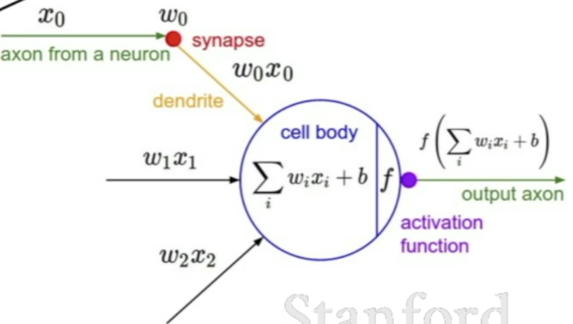
Synapse connects Multiple Neurons -
Dendrites integrate all the information together in cell body -
Output carried on the Output Layer -

충격 발ㄷ언.. Neurons act most similarly to ReLUs... (ReLU non-linearity)