
01. 개요
ML 개념 학습 이후 실전 데이터에 적용해보기 위해 kaggle 컴피티션을 몇 가지 진행한 이후,
hyper-parameter 튜닝 학습을 위한 데이터를 찾던 중 본 대회를 진행해보았다.
(마침, 시계열 데이터도 다뤄보고 싶었고 dacon도 해보고 싶었다.)
[배경]
안정적이고 효율적인 에너지 공급을 위해서는 전력 사용량에 대한 정확한 예측이 필요합니다.
따라서 한국에너지공단에서는 전력 사용량 예측 시뮬레이션을 통한 효율적인 인공지능 알고리즘 발굴을 목표로 본 대회를 개최합니다.
[주제]
전력사용량 예측 AI 모델 개발
[설명]
건물 정보와 시공간 정보를 활용하여 특정 시점의 전력 사용량을 예측하는 AI 모델을 개발해주세요.
[주최 / 주관]
주최: 한국에너지공단
주관: 데이콘
[참가 대상]
데이커라면 누구나
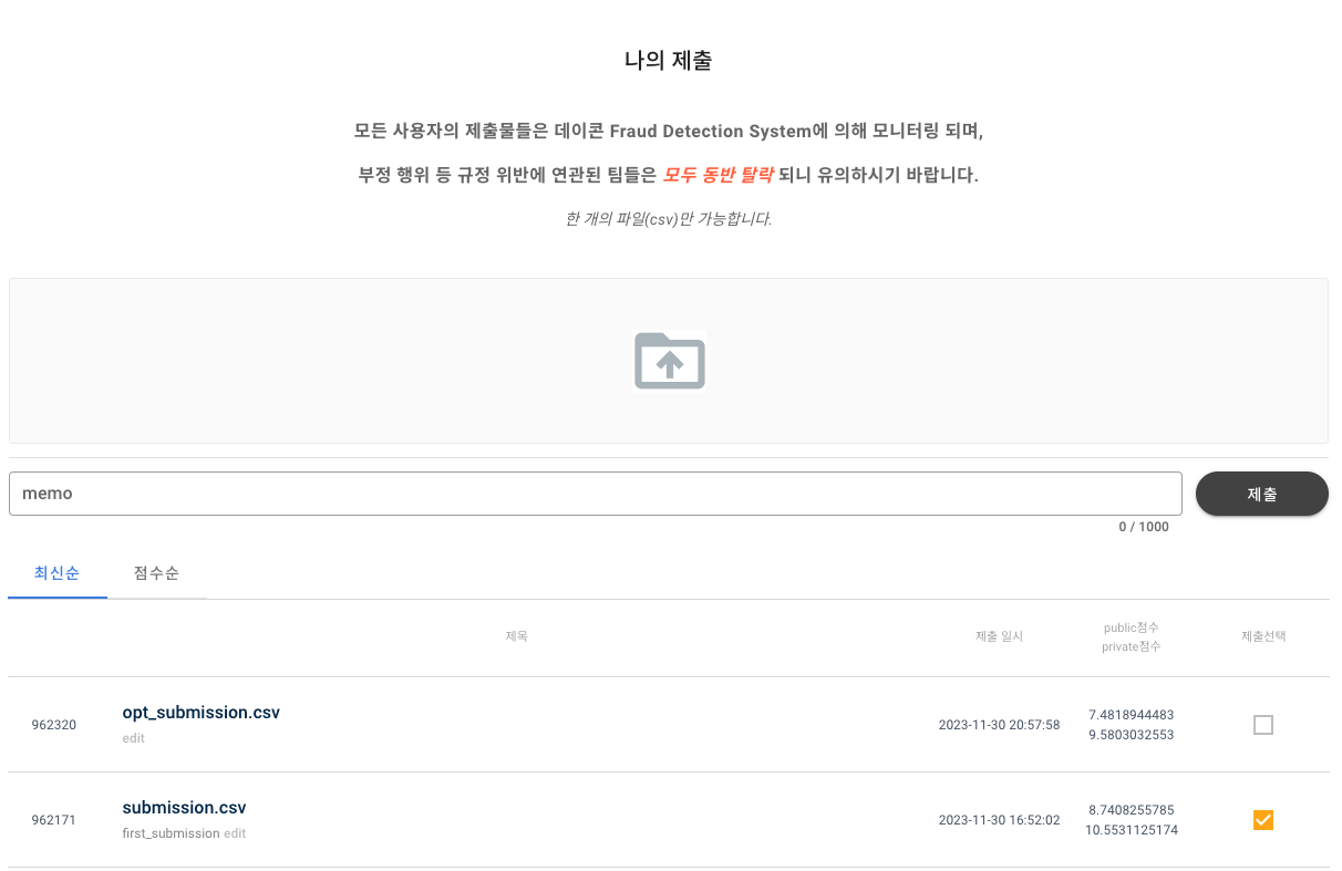
제출은 submission.csv, opt_submission.csv로 두 번 제출하였으며 각각, Light GBM 모델의 hyper-parameter 튜닝 전/후의 결과 파일이다.
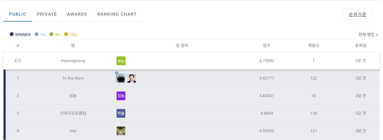
<submission.csv>
<opt_submission.csv>
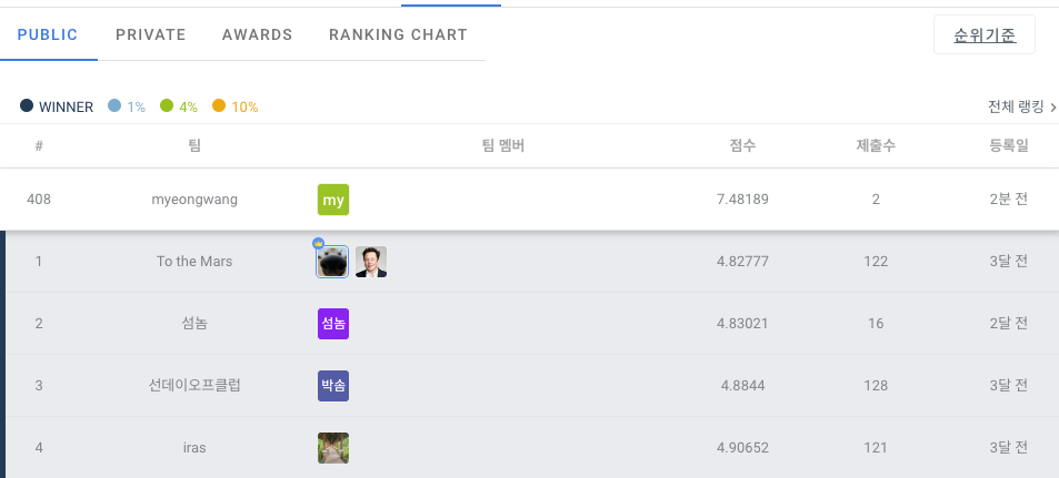
hyper-parameter 튜닝 이전 1233여개의 팀 중 478등 , 튜닝 이후 408등으로 소폭 상승하였다.
(private으로 치면 390등대까지 나왔다.)
02. 라이브러리 및 데이터 불러오기
import numpy as np
import pandas as pd
import matplotlib.pyplot as plt
import seaborn as sns
import optuna

# 모델 성능 평가
from lightgbm.sklearn import LGBMRegressor  # sklearn API
from sklearn.model_selection import train_test_split
from sklearn.metrics import mean_absolute_error
from sklearn.cluster import KMeans

# KFold(CV), partial : optuna를 사용하기 위함
from sklearn.model_selection import KFold
from functools import partial
모델은 LGBM을 적용했다.
# 데이터를 불러옵니다.
base_path = '/Users/myeongjinlee/Desktop/kaggle/kaggle/전력사용예측/'
train = pd.read_csv(base_path + 'train.csv')
building_info = pd.read_csv(base_path + 'building_info.csv')
test = pd.read_csv(base_path + 'test.csv')
print(train.shape, building_info.shape, test.shape)
colab 쓰기 싫어서 로컬에 제공된 데이터를 저장하고 불러왔다.
03. EDA
column 설명
- numdate_time(Primary Key) : 건물번호시간
- 건물번호 : 1 ~ 100
- 일시 : 시간
- 기온, 강수량, 풍속, 습도, 일조, 일사 : 기상정보
- 전력소비량(target) : 건물별 시간당 전력소비량
train.info(memory_usage='deep') #deep 모드로 설정하면, 데이터프레임의 메모리 사용량을 정확하게 파악<class 'pandas.core.frame.DataFrame'>
RangeIndex: 204000 entries, 0 to 203999
Data columns (total 10 columns):
# Column Non-Null Count Dtype
--- ------ -------------- -----
0 num_date_time 204000 non-null object
1 건물번호 204000 non-null int64
2 일시 204000 non-null object
3 기온(C) 204000 non-null float64
4 강수량(mm) 43931 non-null float64
5 풍속(m/s) 203981 non-null float64
6 습도(%) 203991 non-null float64
7 일조(hr) 128818 non-null float64
8 일사(MJ/m2) 116087 non-null float64
9 전력소비량(kWh) 204000 non-null float64
dtypes: float64(7), int64(1), object(2)
memory usage: 39.5 MBtest.info(memory_usage='deep')<class 'pandas.core.frame.DataFrame'>
RangeIndex: 16800 entries, 0 to 16799
Data columns (total 7 columns):
# Column Non-Null Count Dtype
--- ------ -------------- -----
0 num_date_time 16800 non-null object
1 건물번호 16800 non-null int64
2 일시 16800 non-null object
3 기온(C) 16800 non-null float64
4 강수량(mm) 16800 non-null float64
5 풍속(m/s) 16800 non-null float64
6 습도(%) 16800 non-null int64
dtypes: float64(3), int64(2), object(2)
memory usage: 2.9 MBbuilding_info.info(memory_usage='deep')<class 'pandas.core.frame.DataFrame'>
RangeIndex: 100 entries, 0 to 99
Data columns (total 7 columns):
# Column Non-Null Count Dtype
--- ------ -------------- -----
0 건물번호 100 non-null int64
1 건물유형 100 non-null object
2 연면적(m2) 100 non-null float64
3 냉방면적(m2) 100 non-null float64
4 태양광용량(kW) 100 non-null object
5 ESS저장용량(kWh) 100 non-null object
6 PCS용량(kW) 100 non-null object
dtypes: float64(2), int64(1), object(4)
memory usage: 28.3 KBtrain = train.drop(columns=['일조(hr)', '일사(MJ/m2)'])신기하게 train에는 있는데 test data에는 일조, 일사량이 없어서 컬럼 drop
train.columns = ['num_date_time', 'num', 'date_time', 'temperature', 'precipitation',
                 'windspeed', 'humidity', 'target']
test.columns = ['num_date_time', 'num', 'date_time', 'temperature', 'precipitation',
                 'windspeed', 'humidity']
building_info.columns = ['num', 'type', 'area', 'cooling_area', 'solar', 'ESS', 'PCS']
dacon은 colum도 한글이라 영어로 바꿔줬다.
train['date_time'] = pd.to_datetime(train['date_time'])datetime으로 형 변환
building_info = building_info.replace('-',0)

for col in ['태양광용량(kW)', 'ESS저장용량(kWh)', 'PCS용량(kW)']:
    building_info[col] = building_info[col].astype(float)
building_info에 있는 '-'를 모두 0으로 바꾸고, dtype을 float로 변경
시각화
plt.figure(figsize=(10,6))
sns.histplot(data=train ,x='target')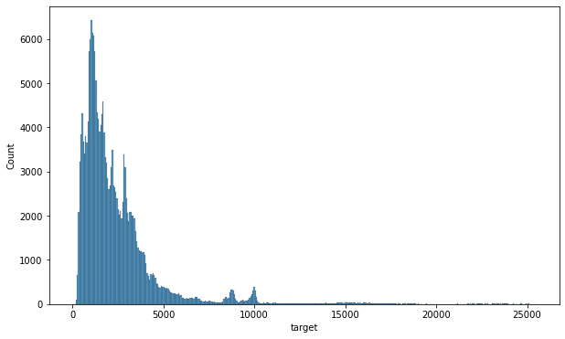
전력 사용량 패턴 분석
plt.figure(figsize=(12,4))
sns.lineplot(data=train, x='date_time', y='target',errorbar=None) 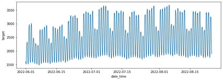
시간변화에 따른 target value(전력사용량) 분석
- 6월보다는 7,8월이 더 높음
- 평일보다 주말이 사용량 낮음 파악
train = pd.merge(train,building_info, on='num' , how ='inner')train에 building_info merge
for bn in train.num.unique():
    plt.figure(figsize=(12, 2))
    plt.title(f'Building {bn}')
    b= train[train.num == bn]
    sns.lineplot(data=b, x="date_time", y='target', errorbar=None)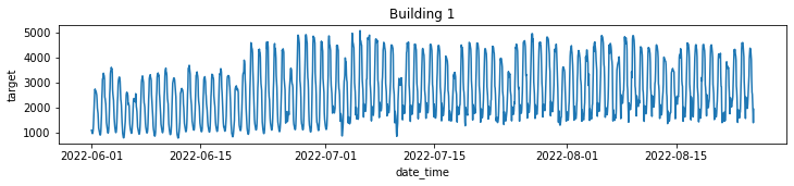
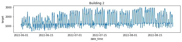
건물 별로 분류해서 각자의 전력사용량 패턴 파악
- 건물 종류별이 아닌 각각의 건물 별로의 분류임(건물 100개니깐 그래프도 100개)
- 예시로 두 개만 업로드
전처리 시 전력사용량 별 건물군집으로 clustering 이후 학습 진행해야겠다는 insight 도출
04. 전처리
결측치 처리
train['precipitation']= train['precipitation'].fillna(0)
train['windspeed']= train['windspeed'].interpolate(method = 'linear')
train['humidity']= train['humidity'].interpolate(method = 'linear')

train.info()<class 'pandas.core.frame.DataFrame'>
Int64Index: 204000 entries, 0 to 203999
Data columns (total 14 columns):
# Column Non-Null Count Dtype
--- ------ -------------- -----
0 num_date_time 204000 non-null object
1 num 204000 non-null int64
2 date_time 204000 non-null datetime64[ns]
3 temperature 204000 non-null float64
4 precipitation 204000 non-null float64
5 windspeed 204000 non-null float64
6 humidity 204000 non-null float64
7 target 204000 non-null float64
8 type 204000 non-null object
9 area 204000 non-null float64
10 cooling_area 204000 non-null float64
11 solar 204000 non-null float64
12 ESS 204000 non-null float64
13 PCS 204000 non-null float64
dtypes: datetime64[ns](1), float64(10), int64(1), object(2)
memory usage: 23.3+ MB
- precipitation(강수량)은 비 온날도 있고 안온날도 있으니 결측치 있는거 그니깐 싹다 0으로 처리
- windspeed, humidity - interpolation(보간법) 적용(어차피 1h 단위인 시계열 데이터니깐)
categorical feature 변환
train = pd.get_dummies(data=train, columns=['type']get_dummies 이용 type 컬럼 one-hot encoding 실시
train['month'] = train.date_time.dt.month
train['day'] = train.date_time.dt.day
train['hour'] = train.date_time.dt.hour
train['dow'] = train.date_time.dt.day_of_week # 0 ~ 6 : 월~일
time feature --> 월/일/시/요일
전력사용량 clustering
cluster_df = pd.DataFrame()

for bn in range(1,101): #1~100
    cluster_df[bn] = train.loc[train.num == bn, 'target'].values

cluster_df = cluster_df.T # 전치
#cluster_df 데이터프레임의 행과 열이 바뀌어서 클러스터링 알고리즘을 적용하기 편한 형태로 데이터 정리
클러스터링 대상:100개( 204000 -> 100 )
- train 데이터프레임에서 num 열의 값이 현재 클러스터링 대상 번호 bn과 일치하는 행을 선택하고, 그 중 'target' 열의 값 가져옴
- 즉, 현재 클러스터링 대상에 해당하는 데이터의 'target' 열 값들을 추출
elbow method 찾기
krange = range(2, 21)
inertias = []
label_list = []
for K in krange:
    km = KMeans(n_clusters=K, n_init=30, random_state=42)
    labels = km.fit_predict(cluster_df) # 100 x 2040
    inertia = km.inertia_

    inertias.append(inertia)
    label_list.append(labels)

plt.figure(figsize=(6, 6))
plt.plot(krange, inertias)
plt.xticks(krange)
plt.show()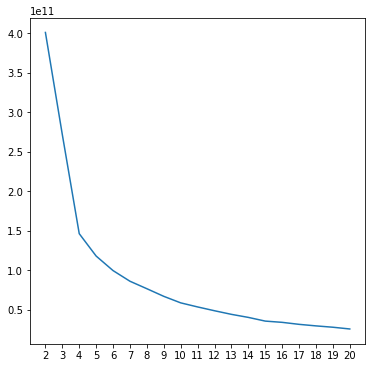
가로 K의 갯수에 따른 inertias 계산 -> 최적의 K = 4 도출
optimal_k = 4
cluster_list = label_list[optimal_k-2] # 시작이 k가 2니깐 인덱스로는 -2 빼줘야지요

cluster_list
array([2, 0, 0, 0, 2, 0, 0, 0, 0, 2, 0, 0, 2, 0, 0, 2, 0, 0, 0, 0, 0, 0,
0, 3, 3, 2, 1, 0, 0, 0, 0, 3, 3, 2, 0, 2, 2, 0, 0, 0, 2, 0, 0, 0,
2, 0, 2, 0, 2, 2, 2, 0, 0, 0, 0, 2, 0, 2, 0, 2, 2, 0, 0, 0, 0, 0,
0, 0, 2, 2, 0, 0, 2, 2, 0, 0, 0, 0, 2, 2, 0, 0, 0, 0, 0, 0, 0, 0,
0, 0, 0, 0, 0, 2, 0, 2, 0, 0, 0, 0], dtype=int32)cluster_df = pd.DataFrame({'num':np.arange(1,101),
'cluster':cluster_list})
train = pd.merge(train, cluster_df, on='num')
train.cluster.value_counts()0 138720
2 55080
3 8160
1 2040
Name: cluster, dtype: int64group 별 데이터 분할
05. 학습 데이터 분할
def data_split(df, num, test_size=0.2, mode='train'):
    if mode == 'train':
        X = df[df.cluster == num].drop(columns=['num_date_time', 'date_time', 'target', 'cluster'])
        y = df[df.cluster == num].target

        X_train, X_val, y_train, y_val = train_test_split(X, y, test_size=test_size, random_state=42)
        print(X_train.shape, y_train.shape, X_val.shape, y_val.shape)
        return X_train, X_val, y_train, y_val

    else: # for test
        X = df[df.cluster == num].drop(columns=['num_date_time', 'date_time', 'cluster'])
        print(X.shape)
        return X
data_split 함수 정의
06. 학습 및 평가
data0 = data_split(train, 0, test_size=0.05)
data1 = data_split(train, 1, test_size=0.05)
data2 = data_split(train, 2, test_size=0.05)
data3 = data_split(train, 3, test_size=0.05)
(131784, 26) (131784,) (6936, 26) (6936,) # X_train, X_val, y_train, y_val
(1938, 26) (1938,) (102, 26) (102,) # X_train, X_val, y_train, y_val
(52326, 26) (52326,) (2754, 26) (2754,) # X_train, X_val, y_train, y_val
(7752, 26) (7752,) (408, 26) (408,) # X_train, X_val, y_train, y_valdata: X_train, X_val, y_train, y_val
model0 = LGBMRegressor(max_depth=12, num_leaves=1023, colsample_bytree=0.5,
                       reg_lambda=5, learning_rate=0.3, n_estimators=100,
                       min_child_samples=20, random_state=42, importance_type='gain') # 104040
model1 = LGBMRegressor(max_depth=5, num_leaves=127, colsample_bytree=0.5,
                       reg_lambda=1, learning_rate=0.3, n_estimators=50,
                       min_child_samples=10, random_state=42, importance_type='gain')# 1530
model2 = LGBMRegressor(max_depth=10, num_leaves=1023, colsample_bytree=0.5,
                       reg_lambda=7, learning_rate=0.23, n_estimators=50,
                       min_child_samples=10, random_state=42, importance_type='gain')# 41310
model3 = LGBMRegressor(max_depth=7, num_leaves=511, colsample_bytree=0.5,
                       reg_lambda=5, learning_rate=0.2, n_estimators=50,
                       min_child_samples=10, random_state=42, importance_type='gain')# 6120
model 적용: LGBMRegressor
LGBM Hyper-parameter 설명
- max_depth (Max Depth): 트리의 최대 깊이 지정
-> 트리의 깊이가 깊을수록 모델은 더 복잡한 패턴을 학습할 수 있지만, 과적합의 위험이 높아짐. - num_leaves (Number of Leaves): 각 트리의 최대 리프 노드(말단 노드)의 개수 지정
-> 트리의 복잡도를 제어하며, 작은 값은 모델의 단순화를 의미하고, 큰 값은 모델의 복잡성을 증가시킴 - colsample_bytree (Column Subsampling by Tree): 각 트리를 구성할 때 열(특성)의 일부만 사용하는 비율을 지정
-> 각 트리를 구성할 때 열(특성)의 일부만 사용하는 비율 지정. 각 트리가 다양한 특성을 학습하고 과적합 방지 - reg_lambda (L2 Regularization Term): L2 정규화 (릿지 정규화)를 적용하는 람다 파라미터
-> 이 값이 크면 모델의 복잡도가 줄어들고, 작으면 모델의 복잡도가 증가. - learning_rate (Learning Rate): 경사 하강법에서 학습률.
-> 이 값은 각 반복 단계에서 모델 파라미터를 업데이트하는 데 사용. 작은 학습률은 안정적인 학습을 보장하지만, 수렴 속도가 느릴 수 있으며, 큰 학습률은 수렴을 빠르게 할 수 있지만 발산할 수 있음. - n_estimators (Number of Estimators): 부스팅 알고리즘에서 생성할 트리의 개수를 지정.
-> 더 많은 트리를 사용하면 모델의 성능이 향상될 수 있지만, 계산 비용이 증가. - min_child_samples (Minimum Number of Samples per Leaf): 각 리프 노드가 가져야 하는 최소 샘플 수를 지정합니다. 이 값을 높이면 트리가 더 단순화되고, 낮추면 모델이 더 복잡한 패턴을 학습할 수 있습니다.
- random_state: 모델의 랜덤 시드(seed)를 지정.
-> 같은 랜덤 시드를 사용하면 모델 학습 시의 무작위성이 재현 가능하며, 결과를 일정하게 만듬. - importance_type: 모델에서 특성 중요도를 계산할 때 사용할 방법을 지정.
def train_and_eval(model, data):
    # data[0] : X_train
    # data[1] : X_val
    # data[2] : y_train
    # data[3] : y_val
    model.fit(data[0], data[2])

    print("Average target value : %.4f" % np.mean(data[2]))
    print("Std target value : %.4f" % np.std(data[2]))
    mean_list = np.mean(data[2]) * np.ones(len(data[2]))
    print("Average absolute error : %.4f" % evaluation_metric(data[2], mean_list))

    print("Prediction")
    pred_train = model.predict(data[0])
    pred_val = model.predict(data[1])

    train_score = evaluation_metric(data[2], pred_train)
    val_score = evaluation_metric(data[3], pred_val)

    print("Train Score : %.4f" % train_score)
    print("Validation Score : %.4f" % val_score)
train 및 validation 지표 출력 함수 생성
train_and_eval(model0, data0)
train_and_eval(model1, data1)
train_and_eval(model2, data2)
train_and_eval(model3, data3)
[LightGBM] [Warning] No further splits with positive gain, best gain: -inf
Average target value : 8964.0107
Std target value : 2176.6939
Average absolute error : 1540.3577
Prediction
Train Score : 119.2221
Validation Score : 131.7465train 및 validation metrics 확인
Hyper-parameter Tuning
def optimizer0(trial, X, y, K):
    # 조절할 hyper-parameter 조합
    num_leaves = trial.suggest_categorical('num_leaves', [2**9-1, 2**10-1, 2**11-1])
    max_depth = trial.suggest_int('max_depth', 10, 15)
    learning_rate = trial.suggest_float('learning_rate', 0.01, 0.1)
    n_estimators = trial.suggest_int('n_estimators', 50, 200)
    min_child_samples = trial.suggest_int('min_child_samples', 10, 25)
    reg_lambda = trial.suggest_float('reg_lambda', 5.0, 20.0)
    colsample_bytree = trial.suggest_categorical('colsample_bytree', [0.5, 0.7])


    # 원하는 모델 지정
    model = LGBMRegressor(num_leaves=num_leaves,
                          max_depth=max_depth,
                          learning_rate=learning_rate,
                          n_estimators=n_estimators,
                          min_child_samples=min_child_samples,
                          reg_lambda=reg_lambda,
                          colsample_bytree=colsample_bytree,
                          random_state=42,
                          verbose=-1)

    # K-Fold Cross validation을 구현
    folds = KFold(n_splits=K, random_state=42, shuffle=True)
    losses = []

    for train_idx, val_idx in folds.split(X, y):
        X_train = X.iloc[train_idx, :]
        y_train = y.iloc[train_idx]

        X_val = X.iloc[val_idx, :]
        y_val = y.iloc[val_idx]

        model.fit(X_train, y_train)
        preds = model.predict(X_val)
        loss = evaluation_metric(y_val, preds)
        losses.append(loss)


    # K-Fold의 평균 loss값을 돌려줍니다.
    return np.mean(losses)
LightGBM 모델의 hyper-parameter 최적화 수행 함수 초기화
- cluster(0,1,2,3) 별로 구분하여 학습 시킬 것이기 때문에 각각의 클러스터에 맞는 하이퍼파라미터 조합 설정 이후 함수 3개 더 정의 ㄱ(예시로 한 개만 업로드)
K = 5   # Kfold 수
opt_func = partial(optimizer0, X=data0[0], y=data0[2], K=K)

study0 = optuna.create_study(direction="minimize") # 최소/최대 어느 방향의 최적값을 구할 건지.
study0.optimize(opt_func, n_trials=30)
최적의 LightGBM 모델 하이퍼파라미터를 찾기 위한 프로세스 자동화. K-Fold 교차 검증을 사용하여 모델의 일반화 성능을 평가하고, Optuna를 통해 최적의 하이퍼파라미터 조합을 찾음.
- trial 30번인데 한 번 하는데 20초 쯤 걸린 듯... 20*30= 600s = 10m
- 마찬가지로 위와 같은 조합 찾기 3번 더 반복(클러스터 별로 각각)
def display_experiments(study):
    print("Best Score: %.4f" % study.best_value) # best score 출력
    print("Best params: ", study.best_trial.params) # best score일 때의 하이퍼파라미터들
    display(study.trials_dataframe())
    optuna.visualization.plot_optimization_history(study)
    optuna.visualization.plot_param_importances(study)
결과 출력 함수 display_experiments 정의
display_experiments(study0)Best Score: 69.6553
Best params: {'num_leaves': 1023, 'max_depth': 15, 'learning_rate': 0.09108662403134193, 'n_estimators': 187, 'min_child_samples': 23, 'reg_lambda': 5.022622949662711, 'colsample_bytree': 0.7}이런 식으로 확인 가능X4
07. 테스트 및 제출파일 생성
submission.csv
- Hyper-parameter 튜닝 미적용
X_test = test.copy()
X_test = pd.merge(X_test, building_info, on='num', how='inner')
X_test = pd.get_dummies(data=X_test, columns=['type'])
X_test.date_time = pd.to_datetime(X_test.date_time)
X_test['month'] = X_test.date_time.dt.month
X_test['day'] = X_test.date_time.dt.day
X_test['hour'] = X_test.date_time.dt.hour
X_test['dow'] = X_test.date_time.dt.day_of_week # 0 ~ 6 : 월~일
X_test = pd.merge(X_test, cluster_df, on='num')
X_test
위에서 train data에 했던 것 처럼 전처리 실시
-  X_test 만들기 : 앞서했던 전처리를 동일하게 적용해주면 됨.
- SQL JOIN (A JOIN B)
- on : 합칠 기준이 되는 column
- how : 'left'(A), 'inner'(A ^ B), 'outer'(A u B)
- 건물 전체를 넣어서 모델링하기 위해 건물 타입을 categorical feature로 변환
- time feature --> 월/일/시/요일
test0 = data_split(X_test, 0, mode='test')
test1 = data_split(X_test, 1, mode='test')
test2 = data_split(X_test, 2, mode='test')
test3 = data_split(X_test, 3, mode='test')
(11424, 26)
(168, 26)
(4536, 26)
(672, 26)4개 모델 각 클러스터 그룹 별 적용
pred0 = model0.predict(test0)
pred1 = model1.predict(test1)
pred2 = model2.predict(test2)
pred3 = model3.predict(test3)
test data에 적용하여 예측
submission = pd.read_csv(base_path + 'sample_submission.csv')
submission
	num_date_time	answer
0	1_20220825 00	0
1	1_20220825 01	0
.
.
.
이런 형태, answer에 예측결과 입력해줘야함.
sample_submission.csv참고하여 submission.csv 파일 생성
submission.loc[test0.index, 'answer'] = pred0
submission.loc[test1.index, 'answer'] = pred1
submission.loc[test2.index, 'answer'] = pred2
submission.loc[test3.index, 'answer'] = pred3
test data 예측값으로 submission.csv 내용 업데이트
num_date_time	answer
0	1_20220825 00	2113.834504
1	1_20220825 01	2032.015726
2	1_20220825 02	1770.983926
3	1_20220825 03	1868.610038
4	1_20220825 04	1822.307221
...	...	...
업데이트 완료.
opt_submission.csv
- Hyper-parameter 튜닝 적용
opt_model0 = LGBMRegressor(
    num_leaves=1023,
    max_depth=15,
    learning_rate=0.09108662403134193,
    n_estimators=187,
    min_child_samples=23,
    reg_lambda=5.022622949662711,
    colsample_bytree=0.7,
    random_state=42
)
위에서 얻은 최적의 파라미터들로 업데이트 X4
X_train0, _, y_train0, _ = data_split(train, 0, test_size=0.2, mode='train')
opt_model0.fit(X_train0, y_train0)
opt_pred0 = opt_model0.predict(test0)
각각의 그룹 별 모델 훈련 및 예측 X4
opt_submission = pd.read_csv(base_path + 'sample_submission.csv')
opt_submission
num_date_time answer
0 1_20220825 00 0
1 1_20220825 01 0
2 1_20220825 02 0
3 1_20220825 03 0
4 1_20220825 04 0
... ... ...sample_submission.csv참고하여 opt_submission.csv 파일 생성
opt_submission.loc[test0.index, 'answer'] = opt_pred0
opt_submission.loc[test1.index, 'answer'] = opt_pred1
opt_submission.loc[test2.index, 'answer'] = opt_pred2
opt_submission.loc[test3.index, 'answer'] = opt_pred3
test data 예측값으로 opt_submission.csv 내용 업데이트
opt_submission num_date_time answer
0 1_20220825 00 2128.532459
1 1_20220825 01 2125.587659
2 1_20220825 02 1888.966095
3 1_20220825 03 1841.722586
4 1_20220825 04 1799.407307
... ... ...
업데이트 완료. The End
08. 제출
< 회고 >
꽤나 재밌지만, 하면 할수록 알아야될게 너무나도 많다는걸 다시 한 번 느낀다...
공부하면 할수록 겸손해진다.
