https://www.kaggle.com/datasets/iarunava/cell-images-for-detecting-malaria

Malaria cell

• 주제 : 말라리아 혈액도말 이미지 분류 실습
• 목적 : TF공식 문서의 이미지 분류를 다른 이미지를 사용해서 응용

1. 이미지 데이터 불러오기 'wget'을 사용하면 온라인 url에 있는 파일을 불러올 수 있다. 논문(혈액도말 이미지로 말라리아 감염여부를 판단하는 논문)에 사용한 데이터셋을 불러옴
2. plt.imread와 CV2(OpenCV)의 imread를 통해 array형태로 데이터를 불러와서 시각화를 해서 감염된 이미지와 아닌 이미지를 비교
3. TF.kera의 전처리 도구를 사용해서 train, valid set을 나눠줌 -> 레이블 값을 폴더명으로 생성해주게 됨

라이브러리 로드

import numpy as np
import pandas as pd
import matplotlib.pyplot as plt

# layers 에서는 Conv2D, MaxPool2D, Dropout, Flatten, Dense 를 불러옵니다.
# callbacks 에서는 EarlyStopping 을 불러옵니다.
import tensorflow as tf
from tensorflow.keras import Sequential
from tensorflow.keras.layers import Conv2D, MaxPool2D, Dropout, Flatten, Dense
from tensorflow.keras.callbacks import EarlyStopping

이미지 다운로드 & 압축 해제

!wget https://data.lhncbc.nlm.nih.gov/public/Malaria/cell_images.zip

!unzip cell_images.zip

import os
for root, dirs, files in os.walk("./cell_images/"):
    print(root, dirs, len(files))

>>>>
./cell_images/ ['Parasitized', 'Uninfected'] 0
./cell_images/Parasitized [] 13780
./cell_images/Uninfected [] 13780

일부 이미지 미리보기

import glob
upics = glob.glob('./cell_images/Uninfected/*.png')
apics = glob.glob('./cell_images/Parasitized/*.png')
len(upics), upics[0], len(apics), apics[0]

>>>>
(13779,
 './cell_images/Uninfected/C174P135NThinF_IMG_20151127_135311_cell_143.png',
 13779,
 './cell_images/Parasitized/C168P129ThinF_IMG_20151118_154126_cell_159.png')

# upics
upics_0 = upics[0]
upics_0_img = plt.imread(upics_0)
plt.imshow(upics_0_img)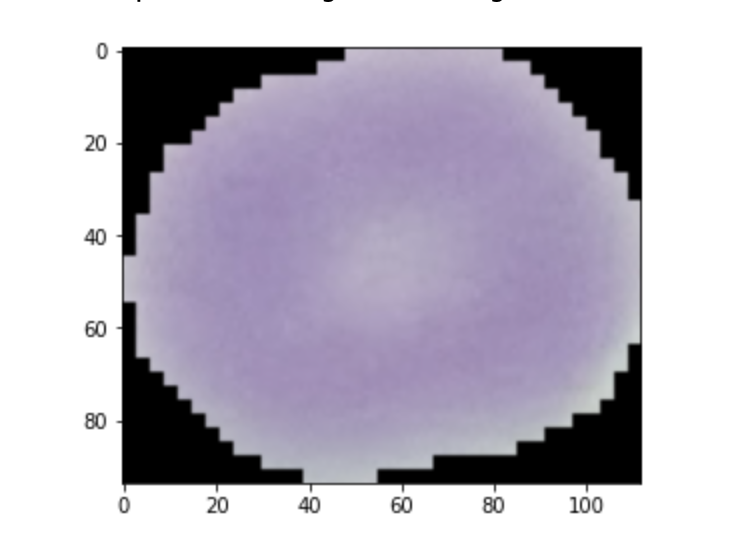

# apics
 apics_0 = apics[0]
 apics_0_img = plt.imread(apics_0)
 plt.imshow(apics_0_img)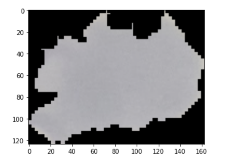

cv2로 시각화

Uninfected

import cv2

plt.figure(figsize=(8, 8))
labels = 'Uninfected'

for i images in enumerate(upics[:9]):
	ax = plt.subplot(3, 3, i+1)
    img = cv2.imread(images)
    plt.imshow(img)
    plt.title(f'{labels} {img.shape}')
    plt.axis('off')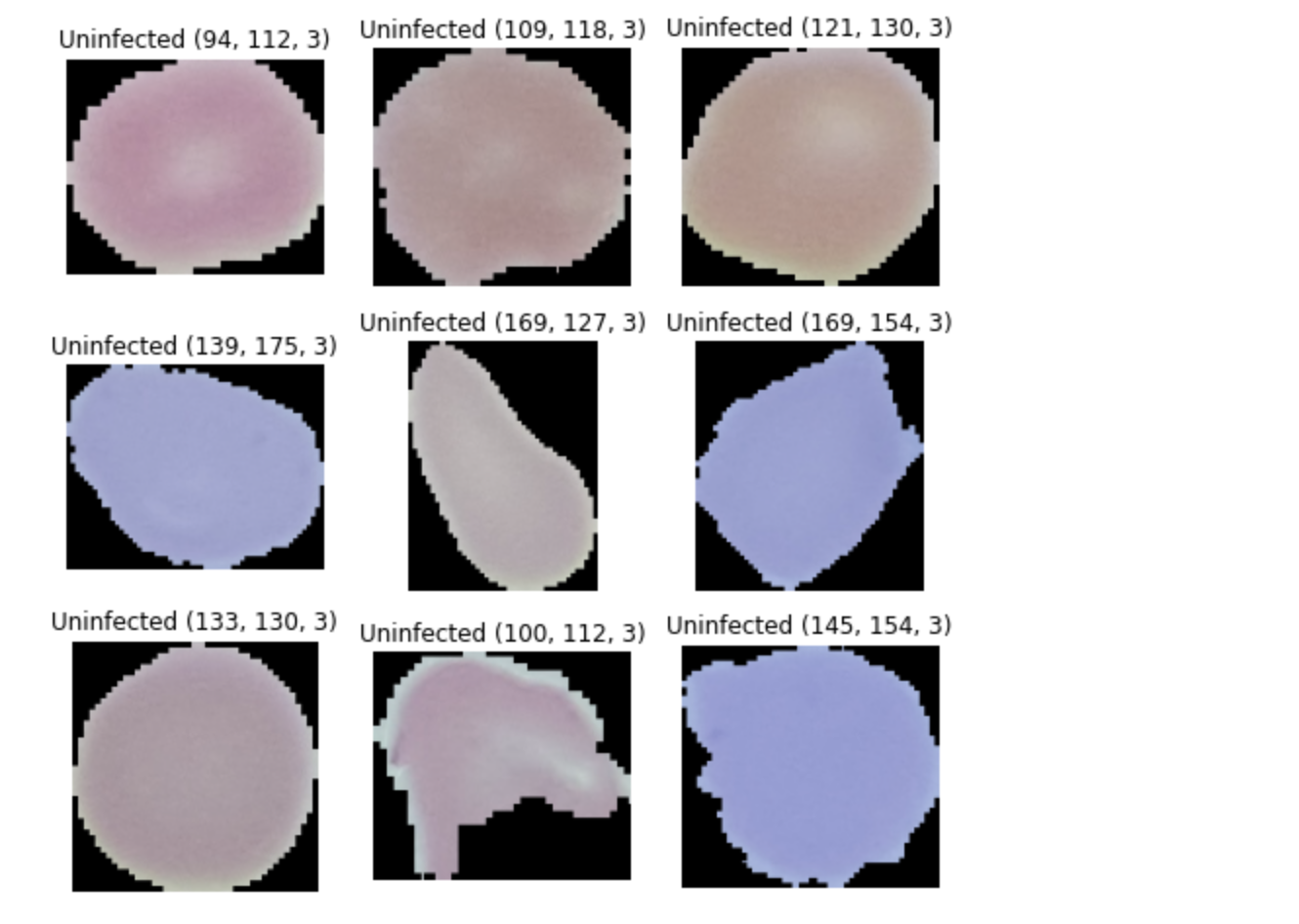

Infected

plt.figure(figsize=(8, 8))
labels = "Infected"

for i, images in enumerate(apics[:9]):
    ax = plt.subplot(3, 3, i + 1)
    img = cv2.imread(images)
    plt.imshow(img)
    plt.title(f'{labels} {img.shape}')
    plt.axis("off")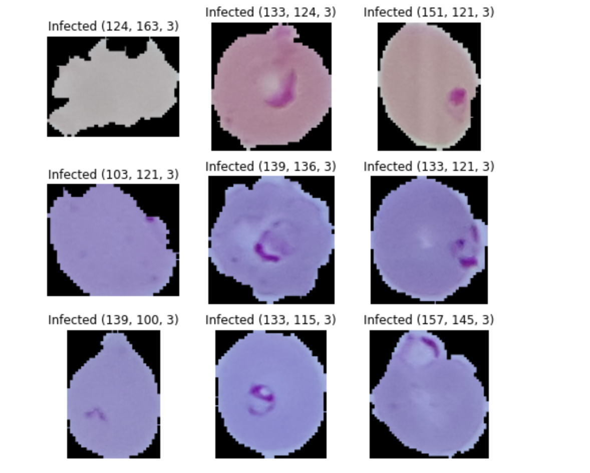

데이터셋 나누기

• 학습, 검증 세트로 나누기
• ImageDataGenerator 통해 이미지를 로드하고 전처리

from tensorflow.keras.preprocessing.image import ImageDataGenerator

#validation_split 값을 통해 학습 : 검증 비율을 8:2로 나눈다
datagen = ImageDataGenerator(rescale=1/255.0, validation_split=0.2)

이미지 사이즈 설정

• 이미지의 사이즈가 불규칙하면 학습을 할 수 없기 때문에 리사이즈할 크기를 지정
• 이미지가 너무 작으면 왜곡되거나 특징을 잃어버릴 수 있다 하지만 계산량이 줄어들어 학습속도가 빠르다.
• 이미지가 너무 크면 흐려지거나 왜곡이 될 수 있으나 좀 더 자세하게 학습할 수도 있다. 하지만 계산량이 많아 학습속도가 오래걸린다.

width=16
height=16

학습 세트

• flow_from_directory 통해 이미지를 불러옵니다.

• training 데이터셋 생성한다.

• class_mode 에는 이진분류이기 때문에 binary 넣어준다

  classmode : One of 'categorical', 'binary', 'sparse',
  'input', or None.
  Default : 'categorical'.
  subset : Subset of data {'training' or 'validation'}
  

trainDatagen = datagen.flow_from_directory(directory = 'cell_images/', 
											target_size = (height, width), 
											class_mode = 'binary', 
											batch_size = 64, 
											subset='training')

>>>>
Found 22048 images belonging to 2 classes.

trainDatagen.num_classes
>>>> 2

trainDatagen.classes
>>>>
array([0, 0, 0, ..., 1, 1, 1], dtype=int32)

# {'Parasitized' : 0, 'Uninfected' : 1}
# 0 : 감염, 1 : 미감염
trainDatagen.class_indices
>>>>
{'Parasitized': 0, 'Uninfected': 1}

검증세트

: validation 데이터셋 생성

valDatagen = datagen.flow_from_directory(directory = 'cell_images/',
                                         target_size =(height, width),
                                         class_mode = 'binary',
                                         batch_size = 64,
                                         subset='validation')

레이어 설정

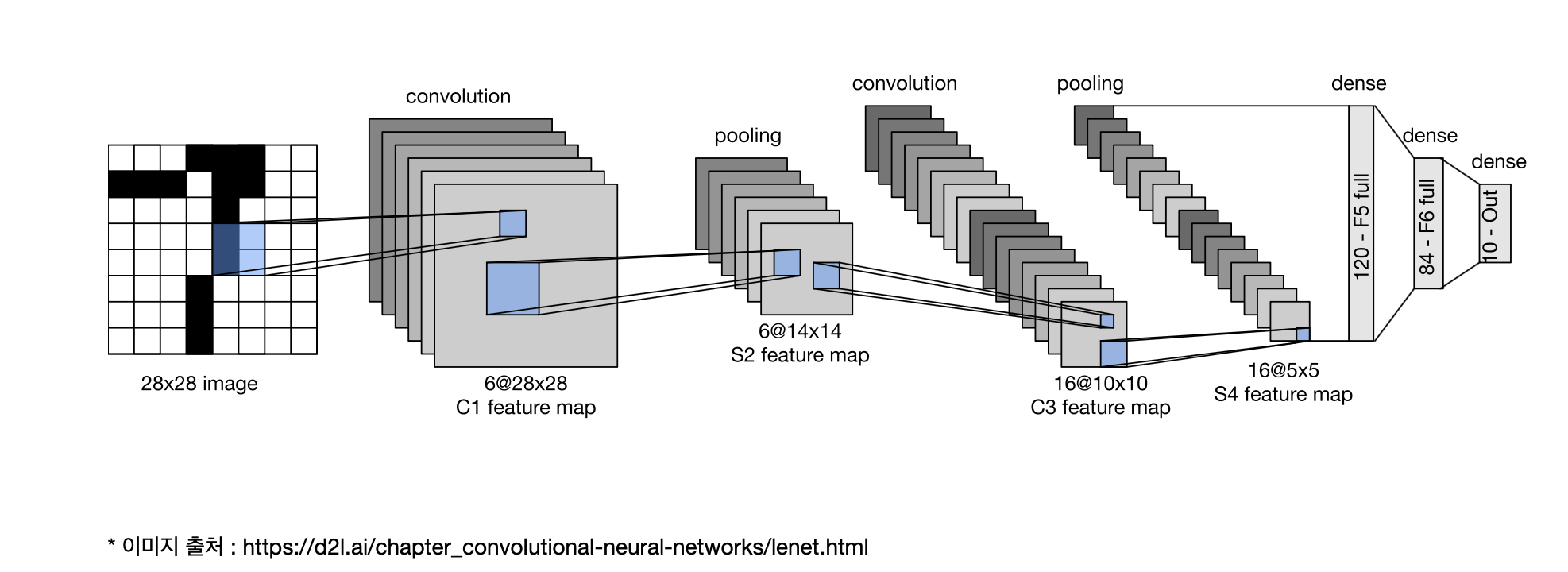
• padding : 경계 처리 방법
  - 'valid' : 유효한 영역만 출력. 따라서 출력 이미지 사이즈는 입력 사이즈보다 작다.
  - 'same' : 출력 이미지 사이즈가 입력 이미지 사이즈와 동일
• input_shape : 모델에서 첫 레이어에서 정의 (height, width, channels)
• activation : 활성화 함수 설정
  - 'linear' : 디폴트 값, 입력 뉴런과 가중치로 계산된 결과값이 그대로 출력
  - 'relu' : rectifier 함수, 은닉층에 주로 사용
  - 'sigmoid' : 시그모이드 함수, 이진 분류 문제에서 출력층에 주로 사용
  - 'softmax' : 소프트맥스 함수, 다중 클래스 분류 문제에서 출력층에 주로 사용
• Dense Layer :
  - 밀집 연결 또는 완전 연결층이라고 불림
  - 첫 번째 Dense층은 128개의 노드를 가진다
  - 마지막 층은 출력층
  • softmax : 2개의 노드의 소프트맥스 층. 이 층은 2개의 확률을 반환하고 반환된 값의 전체 합은 1이다.
  • sigmoid : 둘 중 하나를 예측할 때 1개의 출력값을 출력. 확률을 받아 임계값 기준으로 True, False로 나눈다.
• Output Layer 출력층
  - 예측 값이 n개 : keras.layers.Dense(n, activation='softmax')
  - 예측 값이 둘 중 하나 : keras.layers.Dense(1, activation='sigmoid')

model = Sequential()
# 입력층
model.add(Conv2D(filters=16, kernel_size=(3,3), padding='valid',
                 activation='relu', input_shape=(height, width, 3)))
model.add(Conv2D(filters=16, kernel_size=(3,3), padding='same',
                 activation='relu'))
model.add(MaxPool2D(pool_size=(2,2), strides=1))


model.add(Conv2D(filters=16, kernel_size=(3,3), padding='same',
                 activation='relu'))
model.add(Conv2D(filters=16, kernel_size=(3,3), padding='same',
                 activation='relu'))
model.add(MaxPool2D(pool_size=(2,2), strides=1))
# 20% 는 0으로 대체합니다. => 오버피팅 방지
model.add(Dropout(0.2))

# Fully-connected layer
model.add(Flatten())
model.add(Dense(units=64, activation='relu'))
model.add(Dense(units=32, activation='relu'))

# 출력층=> binary classification
model.add(Dense(1, activation='sigmoid'))

# summary
model.summary()

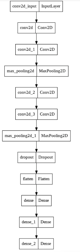
# tensorflow.keras.utils의 plot_model 을 통한 레이어 시각화
from tensorflow.keras.utils import plot_model

plot_model(model)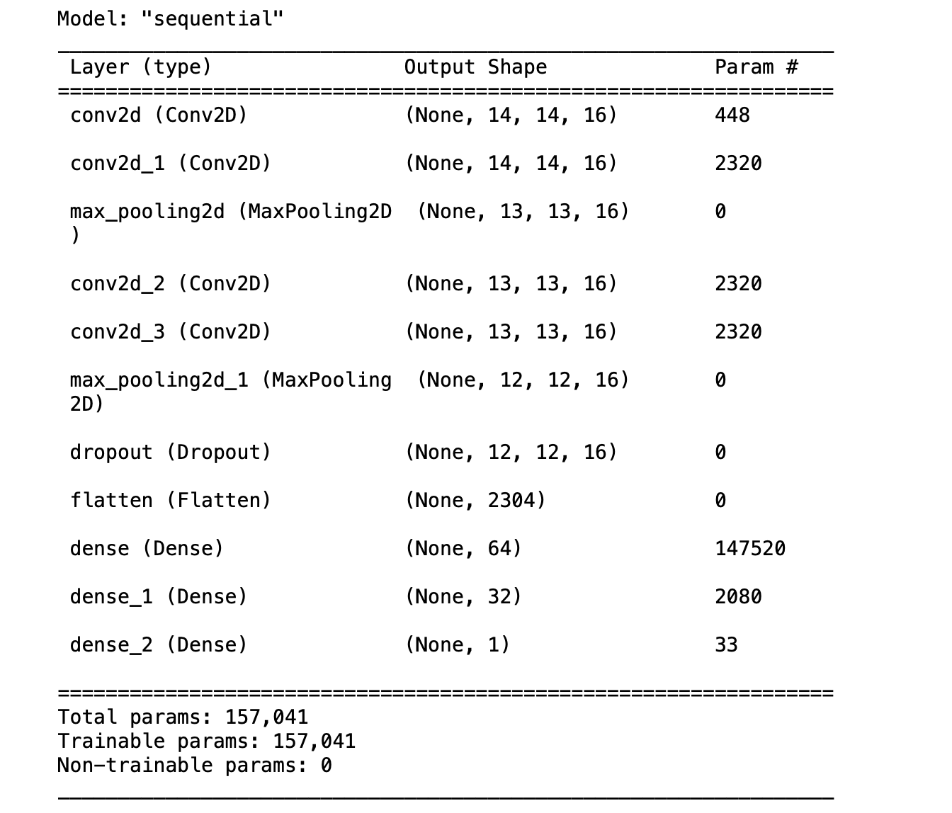

compile

model.complie(optimizer='adam', 
				loss='binary_crossentropy', 
                metrics=[accuracy'])

학습 (fit)

배치(batch): 모델 학습에 한 번에 입력할 데이터셋
에폭(epoch): 모델 학습시 전체 데이터를 학습한 횟 수
스텝(step): (모델 학습의 경우) 하나의 배치를 학습한 횟 수
EarlyStopping: 성능이 더 이상 좋아지지 않으면 학습을 중지
early_stop = EarlyStopping(monitor='val_loss', patience=2)

early_stop = EarlyStopping(monitor='val_loss', patience=5)

# fit
history = model.fit(trainDatagen, epochs=1000, validation_data=valDatagen, callbacks=early_stop)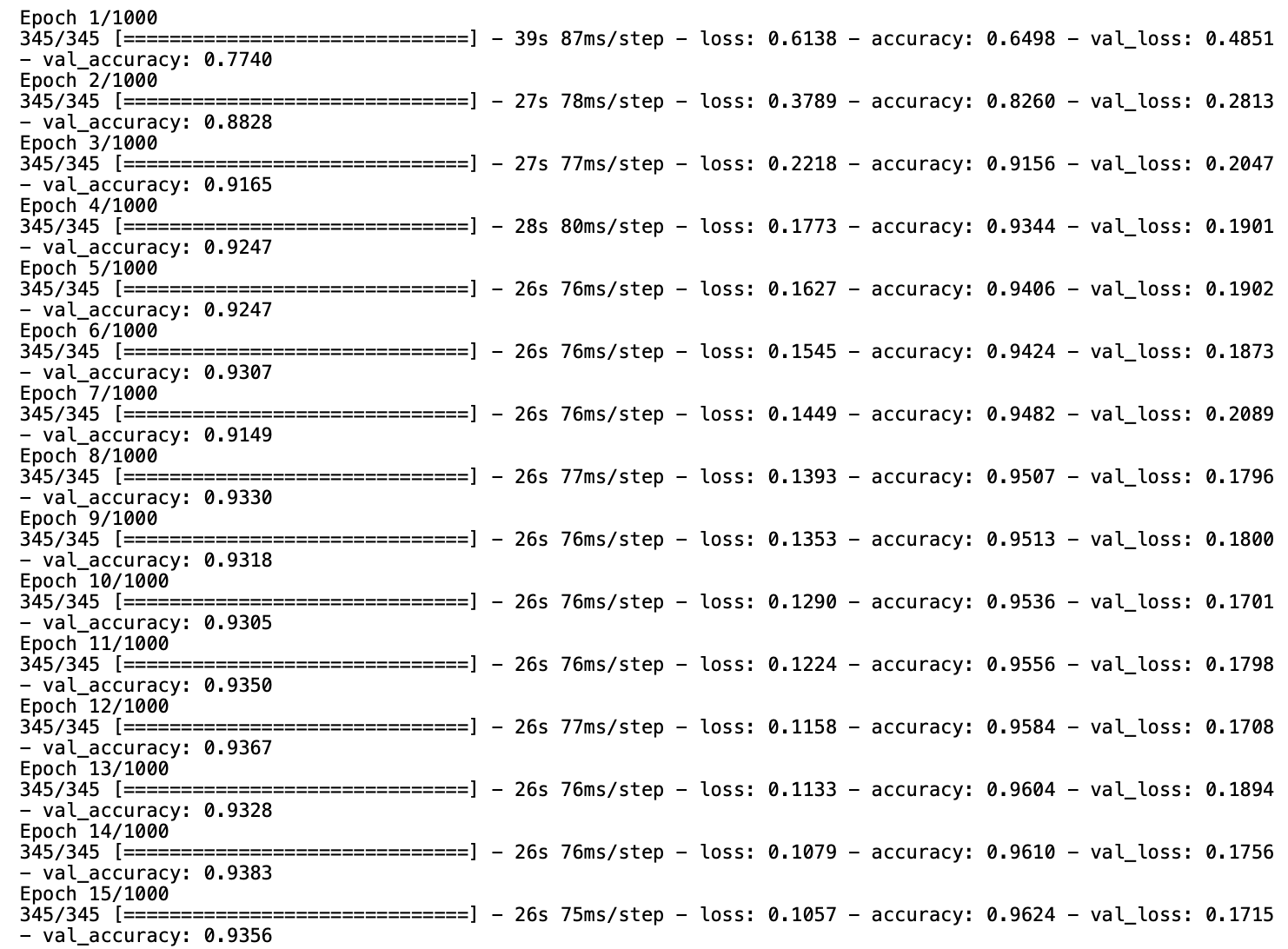

# history
df_hist = pd.DataFrame(history.history)
df_hist.tail()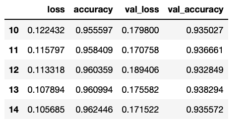

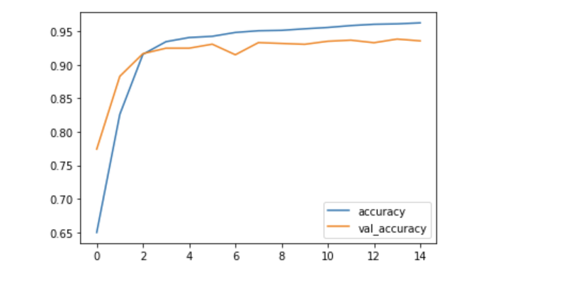
학습결과 시각화

df_hist[['loss', 'val_loss']].plot()
df_hist[['accuracy', 'val_accuracy']].plot()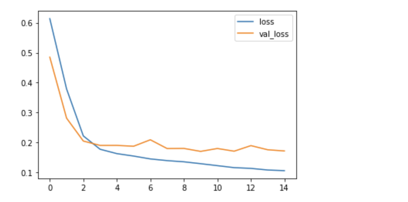