https://www.kaggle.com/datasets/vijaygiitk/multiclass-weather-dataset

Weather Classification

The dataset contains 6-folders: 5-folders having each category of images and one with the alien-test having the images of all categories. It also consist a csv file having the labels for the images in alien-test folder.

• colab 실습

라이브러리 로드

import numpy as np
import pandas as pd
import matplotlib.pyplot as plt
import seaborn as sns
import random
import os
import tqdm as tqdm
import cv2

이미지 로드

# mount
from google.colab import drive
drive.mount('/gdrive')

with open('/gdrive/My Drive/data/dataset2', 'w') as f:
  f.write('Hello Google Drive!')
!cat '/gdrive/My Drive/data/dataset2'

!unzip archive.zip

정답값 폴더명

import os
root_dir = '/gdrive/My Drive/data/dataset'
image_label = os.listdir(root_dir)
image_label.remove('test.csv')
image_label
>>>>
['cloudy', 'shine', 'rainy', 'alien_test', 'foggy', 'sunrise']

일부 이미지 미리보기

import glob 
fig, axes = plt.subplots(nrow=1, ncols=len(image_label), figsize=(20, 5))

for i, img_label in enumerate(image_label):
	wfiles = glob.glob(f"{root_dir}/{img_label}/*")
    wfiles = sorted(wfiles)
    print(wfiles[0])
    img = plt.imread(wfiles[1])
    axes[i].imread(img)
    axes[i].set_title(img_label)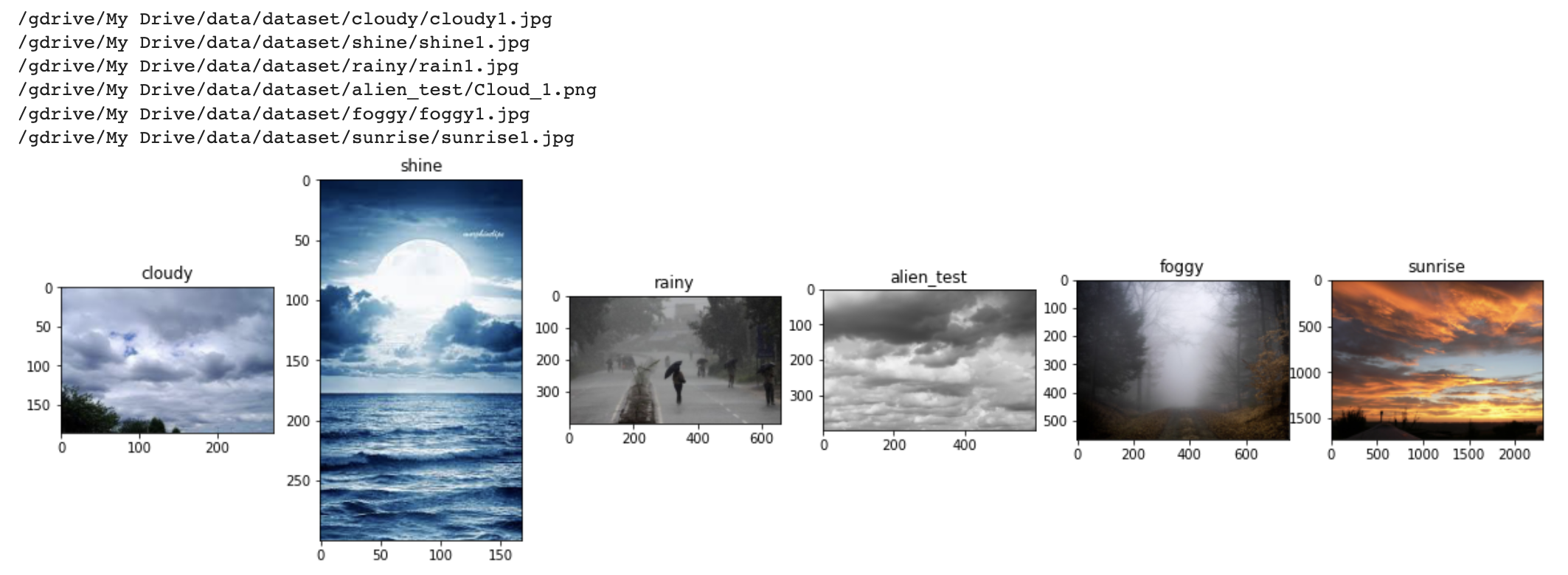

이미지 데이터셋 만들기

def img_read_resize(img_path):
	img = cv2.imread(img_path)
    img = cv2.cvtColor(img, cv2.COLOR_BGR2RGB)
    img = cv2.resize(img, (120, 120))
    return img

img_path = f"{root_dir}/cloudy/cloudy131.jpg"
print(img_read_resize(img_path).shape)

# 이미지 사이즈 변경 확인
plt.imread(img_resize(img_path))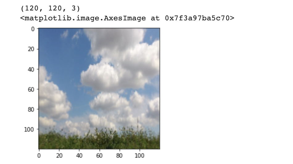

전체 이미지 파일을 list에

• 특정 날씨 폴더의 전체 이미지를 읽어온다
• 반복문을 통해 이미지를 하나씩 순회하며 imread 로 배열 형태로 변경된 이미지를 읽어온다
• img_files 리스트에 읽어온 이미지를 append 로 하나씩 추가
• 반복문 순회가 끝나면 img_files 리스트로 변환
• 형식에 맞지 않는 이미지를 제외하고 가져오도록 try, except 사용

def img_folder_read(img_label):
	img_files = []
    labels = []
    wfiles = glob.glob(f"{root_dir}/{img_label}/*")
    wfiles = sorted(wfiles)
    for w_img in wfiles:
    	try:
        	img_files.append(img_read_resize(w_img))
            labels.append(img_label)
        except:
        	continue
   return img_files, labels

img_label = 'shine'
img_files, labels = img_folder_read(img_label)
len(img_files), len(labels), img_files[0].shape, labels[0]

>>>>
(249, 249, (120, 120, 3), 'shine')

image_label
>>>>
['cloudy', 'shine', 'rainy', 'alien_test', 'foggy', 'sunrise']

x_train_img = []
x_test_img = []
y_train_img = []
y_test_img = []

for img_label in tqdm.tqdm(image_label):
	x_temp, y_temp = img.folder_read(img_label)
    if img_label == 'alien_test':
    	x_test_img.extend(x_temp)
        y_test_img.extend(y_temp)
    else:
    	x_train_img.extend(x_temp)
        y_train_img.extend(y_temp)

len(x_train_img), len(y_train_img), len(x_test_img), len(y_test_img)
>>>>
100%|█ █ █ █ █ █ █ █ █ █| 6/6 [00:22<00:00,  3.68s/it]
(1498, 1498, 30, 30)

# train 데이터 미리보기
plt.imshow(x_train_img[170])
plt.title(y_train_img[170])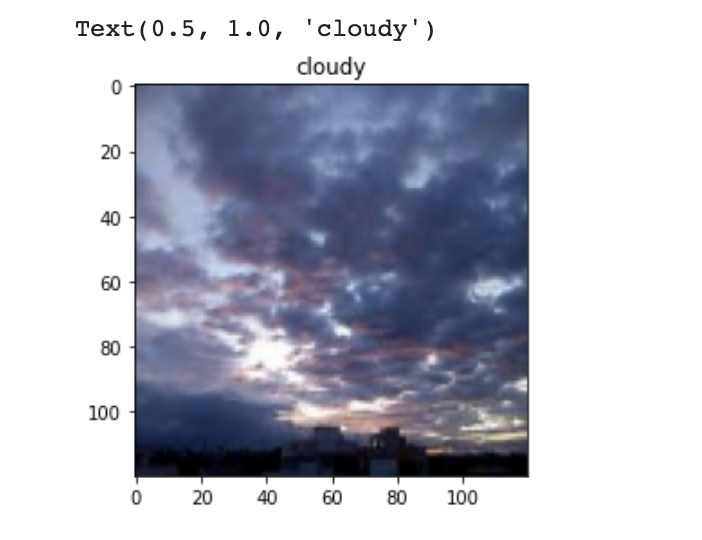

# test 데이터 미리보기
plt.imshow(x_test_img[6])
plt.title(y_test_img[0])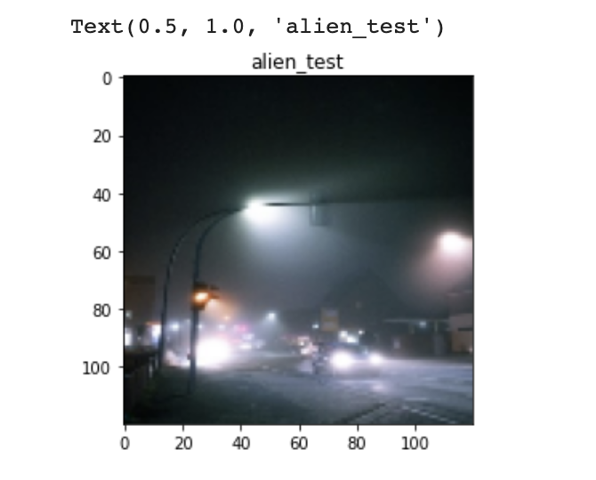

x, y 값 np.array 형식 만들기

• 기존의 데이터가 리스트 형태이기 때문에 numpy 배열 형태로 변경
• train, valid, test set에 대한 X, y값 만들기
• label 별로 각 폴더의 파일의 목록을 읽어오기
• 이미지와 label 리스트를 만들어서 넣어준다
• test는 폴더가 따로 있어서 이미지 불러올 때 test 여부를 체크하여 train, test를 먼저 만든다
• np.array 형태로 변환
• train으로 train, valid를 나누어 준다.
• train, valid, test를 만들어준다.

x_train_arr = np.array(x_train_img)
y_train_arr = np.array(y_train_img)
x_test_arr = np.array(x_test_img)
y_test_arr = np.array(y_test_img)

x_train_arr.shape, y_train_arr.shape, x_test_arr.shape, y_test_arr.shape
>>>>
((1498, 120, 120, 3), (1498,), (30, 120, 120, 3), (30,))

train, valid 나누기

• train_test_split
• class가 균일하게 나누어지지 않아 학습이 불균형하게 되는 문제를 해결
• valid 데이터를 직접 나눠주면 좀 더 잘 학습

from sklearn.model_selection import train_test_split
x_train_raw, x_valid_raw, y_train_raw, y_valid_raw = train_test_split(
	x_train_arr, y_train_arr, test_size=0.33, random_state=42, stratify=y_train_arr)
    
x_train_raw.shape, x_valid_raw.shape, y_train_raw.shape, y_valid_raw.shape
>>>>
((1003, 120, 120, 3), (495, 120, 120, 3), (1003,), (495,))

이미지 데이터 정규화

• R, G, B는 0~255로 3개의 빨, 초, 파로 표현

x_train = x_train_raw / 255
x_valid = x_valid_raw / 255
x_test = x_test_arr / 255

x_train[0].max(), x_valid[0].max(), x_test[0].max()
>>>>
(1.0, 1.0, 1.0)

One-Hot-Encoding

• LabelBinarizer()
  : 'cloudy', 'shine', 'sunrise', 'rainy', 'foggy' 형태의 분류를 숫자로 변경
• y_test는 정답값 비교를 할 예정이므로 학습에 사용하지 않기 때문에 인코딩 하지 않아도 됨

y_train_arr
>>>>
array(['cloudy', 'cloudy', 'cloudy', ..., 'sunrise', 'sunrise', 'sunrise'],
      dtype='<U7')
      
from sklearn.preprocessing import LabelBinarizer

lb = LabelBinarizer()
lb.fit(y_train_arr)
print(lb.classes_)
y_train = lb.transform(y_train_raw)
y_valid = lb.transform(y_valid_raw)

y_train.shape, y_valid.shape
>>>>
['cloudy' 'foggy' 'rainy' 'shine' 'sunrise']
((1003, 5), (495, 5))

정답 빈도수

lb.classes_
>>>>
array(['cloudy', 'foggy', 'rainy', 'shine', 'sunrise'], dtype='<U7')

# 정답 인코딩이 제대로 되어있는지 확인
# 클래스가 train, valid 균일하게 나눠졌는지 확인
# pd.Series 형태로 구성해 준 이유는 np.array 형태이기 때문
pd.Series(y_train_raw).value_counts(1)
>>>>
sunrise    0.233300
cloudy     0.200399
foggy      0.200399
rainy      0.199402
shine      0.166500
dtype: float64

pd.Series(y_valid_raw).value_counts(1)
>>>>
sunrise    0.234343
rainy      0.200000
cloudy     0.200000
foggy      0.200000
shine      0.165657
dtype: float64

층 구성

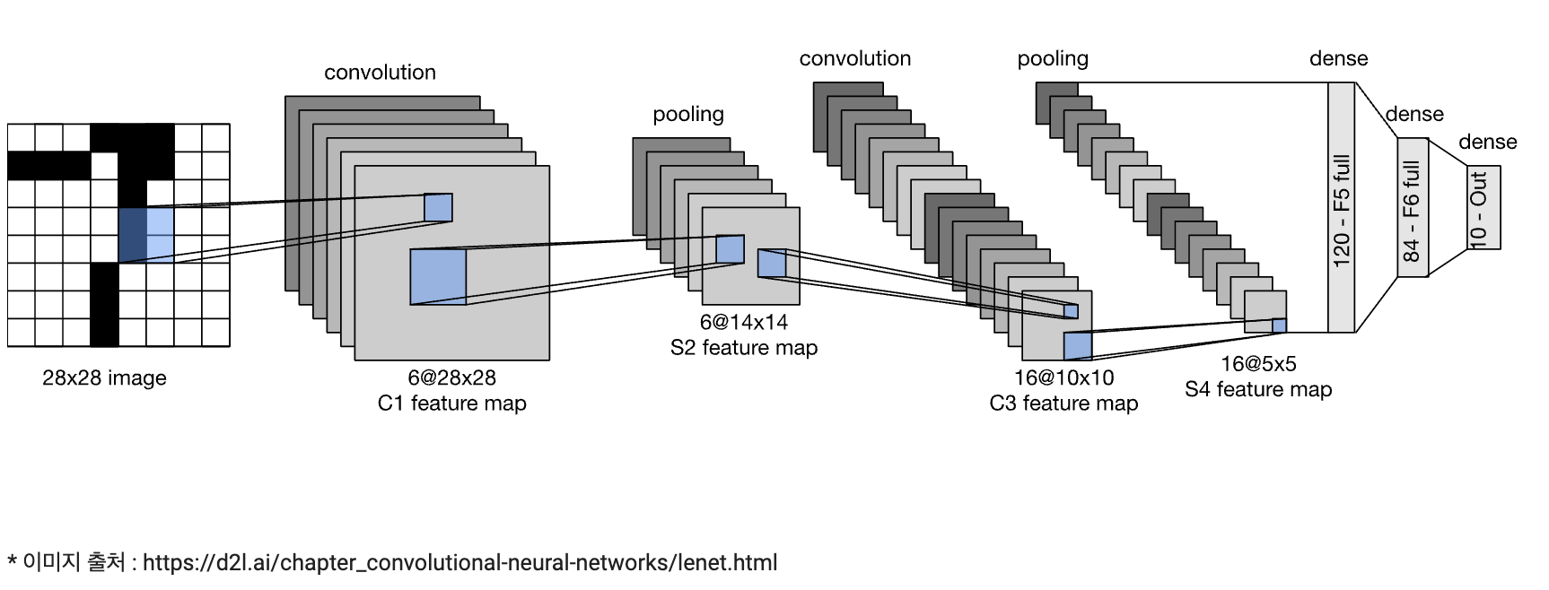
from tensorflow.keras.models import Sequential
from tensorflow.keras.layers import Conv2D, MaxPool2D, Dense, Flatten, Dropout

y_train.shape
>>>>
(1003, 5)

# 예측할 class의 수가 shape의 열의 개수가 된다. 
n_class = y_train.shape[1]
n_class
>>>>
5

layers 구성

model = Sequential()

model.add(Conv2D(filter=16, kernel_size=(3, 3),
			activation='relu', input_shape=x_train[o].shape))
model.add(MaxPool2D(2, 2))
model.add(Dropout(0.2))

model.add(Conv2D(filters=64, kernel_size=(3,3), padding='same',
                 activation='relu'))
model.add(MaxPool2D(pool_size=(2,2), strides=1))
model.add(Dropout(0.2))

# Flatten => 1차원 형태로 변환하고 Fully-connected Layer로 전달하기 위해
model.add(Flatten())
model.add(Dense(units=64, activation="relu"))
model.add(Dense(units=32, activation='relu'))

# 출력층
model.add(Dense(n_class, activation='softmax'))

summary

model.summary()

>>>>
Model: "sequential_25"
_________________________________________________________________
 Layer (type)                Output Shape              Param #   
=================================================================
 conv2d_26 (Conv2D)          (None, 118, 118, 16)      448       
                                                                 
 max_pooling2d_26 (MaxPoolin  (None, 59, 59, 16)       0         
 g2D)                                                            
                                                                 
 dropout_23 (Dropout)        (None, 59, 59, 16)        0         
                                                                 
 conv2d_27 (Conv2D)          (None, 59, 59, 64)        9280      
                                                                 
 max_pooling2d_27 (MaxPoolin  (None, 58, 58, 64)       0         
 g2D)                                                            
                                                                 
 dropout_24 (Dropout)        (None, 58, 58, 64)        0         
                                                                 
 flatten_12 (Flatten)        (None, 215296)            0         
                                                                 
 dense_38 (Dense)            (None, 64)                13779008  
                                                                 
 dense_39 (Dense)            (None, 32)                2080      
                                                                 
 dense_40 (Dense)            (None, 5)                 165       
                                                                 
=================================================================
Total params: 13,790,981
Trainable params: 13,790,981
Non-trainable params: 0
_________________________________________________________________

compile

model.compile(optimizer='adam', 
				loss='categorical_crossentropy', 
                metrics=['accuracy']
                )

fit

from tensorflow.keras.callbacks import EarlyStopping
earlystop = EarlyStopping(monitor="val_accuracy", patience=5, verbose=1)

history = model.fit(x_train, y_train, validation_data=(x_valid, y_valid), 
                    epochs=20, callbacks=[earlystop])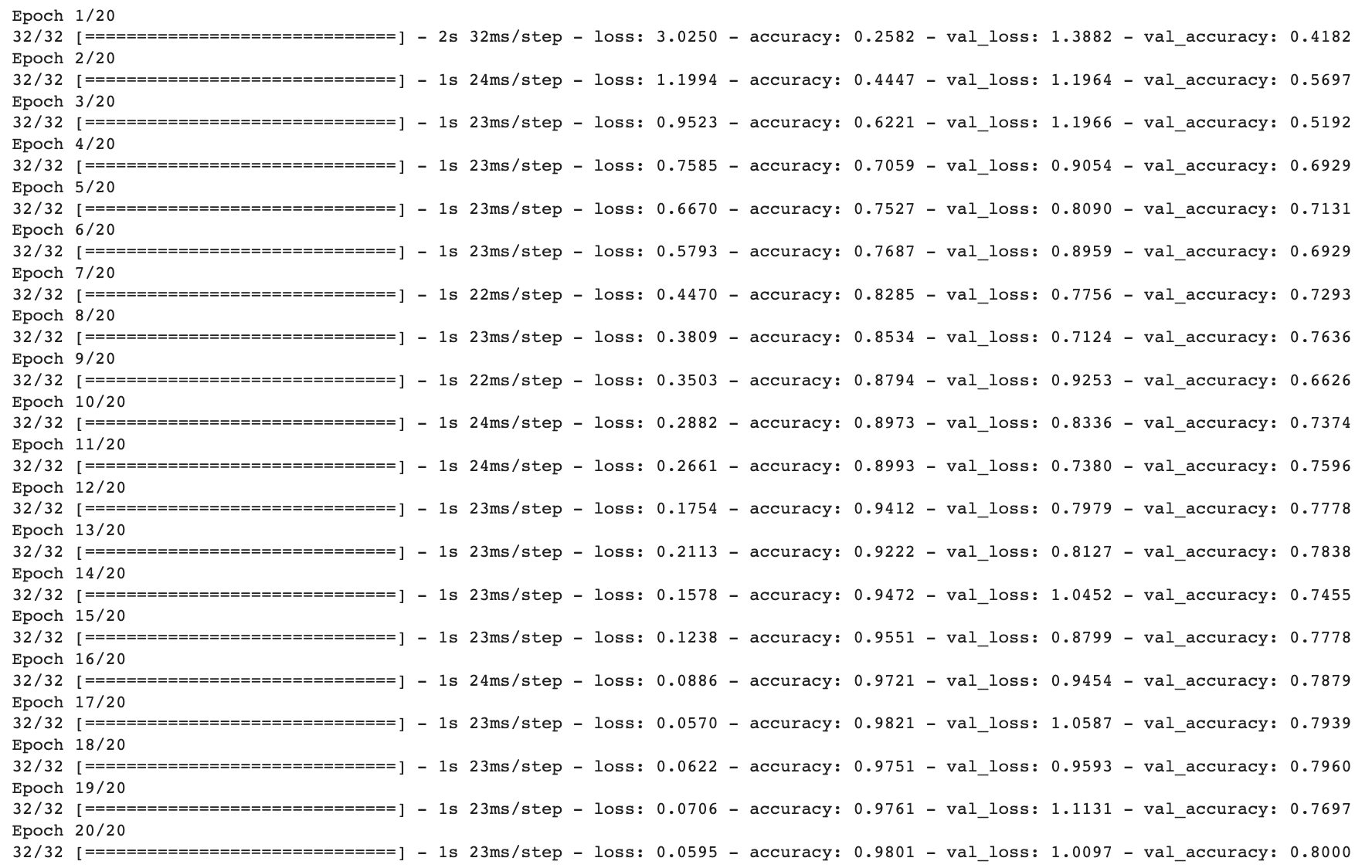

history

df_hist = pd.DataFrame(history.history)
df_hist.tail
>>>>
<bound method NDFrame.tail of         
		loss  accuracy  val_loss  val_accuracy
0   3.025001  0.258225  1.388153      0.418182
1   1.199404  0.444666  1.196450      0.569697
2   0.952285  0.622134  1.196582      0.519192
3   0.758515  0.705882  0.905438      0.692929
4   0.666997  0.752742  0.809039      0.713131
5   0.579274  0.768694  0.895901      0.692929
6   0.446963  0.828514  0.775644      0.729293
7   0.380925  0.853440  0.712370      0.763636
8   0.350297  0.879362  0.925306      0.662626
9   0.288178  0.897308  0.833619      0.737374
10  0.266054  0.899302  0.738016      0.759596
11  0.175380  0.941176  0.797875      0.777778
12  0.211277  0.922233  0.812663      0.783838
13  0.157780  0.947159  1.045204      0.745455
14  0.123782  0.955135  0.879894      0.777778
15  0.088632  0.972084  0.945401      0.787879
16  0.057009  0.982054  1.058660      0.793939
17  0.062206  0.975075  0.959297      0.795960
18  0.070612  0.976072  1.113115      0.769697
19  0.059526  0.980060  1.009745      0.800000>

시각화

df_hist[['accuracy', 'val_accuracy']].plot()

df_hist[['loss', 'val_loss']].plot()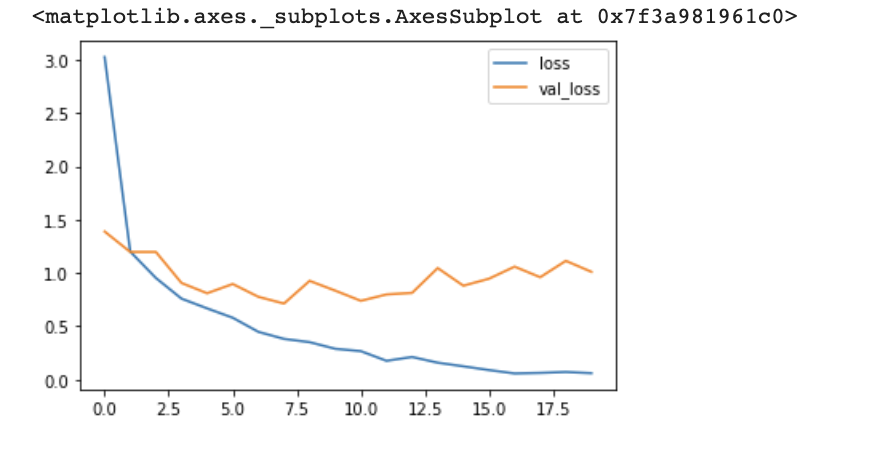

predict

# softmax로 출력했기 때문에 합이 1이 되는 값으로 출력

y_pred = model.predict(x_test)
y_pred[0]
>>>>
array([4.6532657e-02, 9.2098981e-01, 3.1598058e-02, 3.0585946e-04,
       5.7366164e-04], dtype=float32)
       

실제값과 예측값 비교

# TF로 예측한 값을 csv파일과 비교
test = pd.read_csv(f'{root_dir}/test.csv')
y_test = test['labels']

y_predict = np.argmax(y_pred, axis=1)
y_predict[:5]
>>>>
array([1, 0, 0, 1, 1])

(y_test == y_predict).mean()
>>>>
0.8

전체 이미지 시각화

test.head()
>>>>
	Image_id	labels
0	Cloud_1.png		0
1	Cloud_2.jpg		0
2	Cloud_3.jpeg	0
3	Cloud_4.jpg		0
4	foggy_1.jpg		1

• 전체 테스트 이미지 시각화
• train의 0은 cloudy인데 test는 rain이 아닌 지 확인 필요
• subplot으로 30개 이미지 한번에 시각화
• row, col을 구해서 해당 위치에 이미지 넣어준다

fig, axes = plt.subplots(nrows=6, ncols=5, figsize=(20, 20))
for i tcsv in test.iterrows():
	col = i % 5
    row = i // 5
    Image_id = tcsv['Image_id']
    img_label = tcsv['labels']
    img = plt.imread(f'{root_dir}/alien_test/{Image_id}')
    
    color = 'red'
    if img_label == y_predict[i]:
    	color = 'blue'
        
   axes[row, col].imshow(img)
   axes[row, col].set_title(f"test : {class_name[img_label]}, predict : {class_name[y_predict[i]]}', color=color)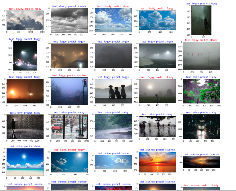