tensorflow 분류 모델 만들기

https://www.tensorflow.org/tutorials/keras/classification

전체 수치변수 시각화

df.hist(figsize=(8, 8))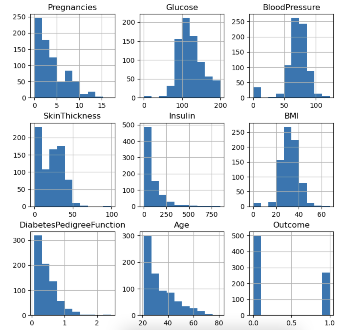

데이터셋 나누기

label_name = 'Outcome'

df.columns
>>>>
Index(['Pregnancies', 'Glucose', 'BloodPressure', 'SkinThickness', 'Insulin',
       'BMI', 'DiabetesPedigreeFunction', 'Age', 'Outcome'],
      dtype='object')
      
# X, y 만들기
X = df.drop(columns=label_name)
y = df[label_name]

X.shape, y.shape
>>>>
((768, 8), (768,))

train_test_split

from sklearn.model_selection import train_test_split

X_train, X_test, y_train, y_test = train_test_split(X, y, test_size=0.2, random_state=42)

X_train.shape, X_test.shape, y_train.shape, y_test.shape
>>>>
((614, 8), (154, 8), (614,), (154,))

tensorflow

import tensorflow as tf

Activation Function

print(dir(tf.keras.activation)[:10])
>>>>
['deserialize', 'elu', 'exponential', 'gelu', 'get',
'hard_sigmoid', 'linear', 'relu', 'selu', 'serialize',
'sigmoid', 'softmax', 'softplus', 'softsign', 'swish', 'tanh']

sigmoid

: 이진분류문제(출력층)

plt.plot(x, tf.keras.activations.sigmoid(x), linestyle='--', label='sigmoid')
plt.axvline(0)
plt.legend()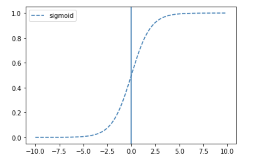

tanh

plt.plot(x, tf.keras.activations.tanh(x), linestyle='--', label='tanh')
plt.axvline(0)
plt.legend()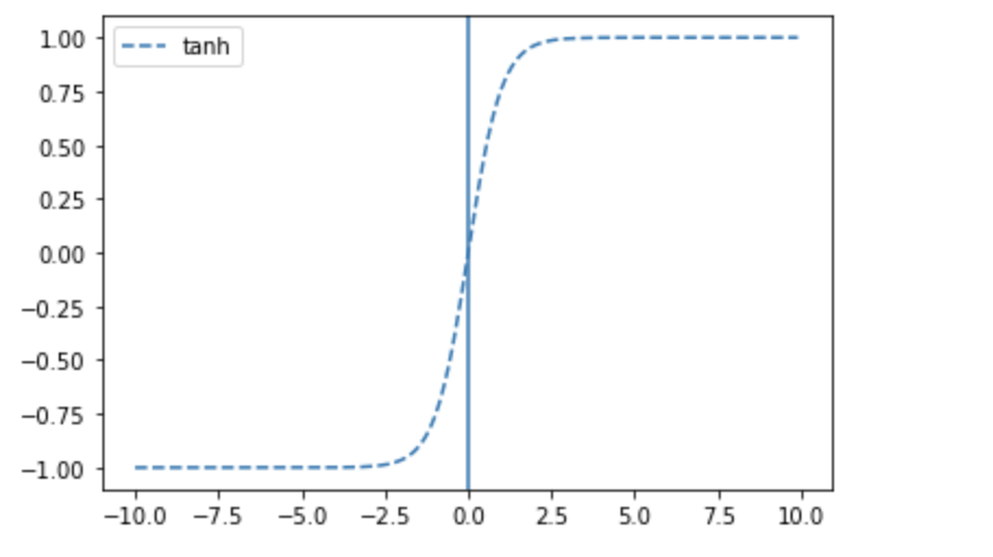

swish

plt.plot(x, tf.keras.activations.swish(x), linestyle='--', label="swish")
plt.axvline(0)
plt.legend()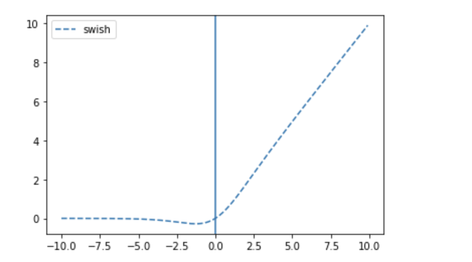

relu

: 은닉층에 주로 사용

plt.plot(x, tf.keras.activations.relu(x), linestyle='--', label="relu")
plt.axvline(0)
plt.legend()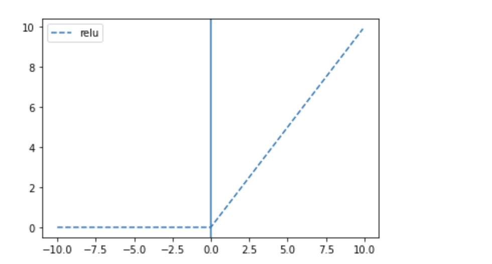

softmax

: 다중 클래스 분류 문제 (출력층)

plt.plot(x, tf.keras.activations.softplus(x), linestyle='--', label="softplus")
plt.axvline(0)
plt.legend()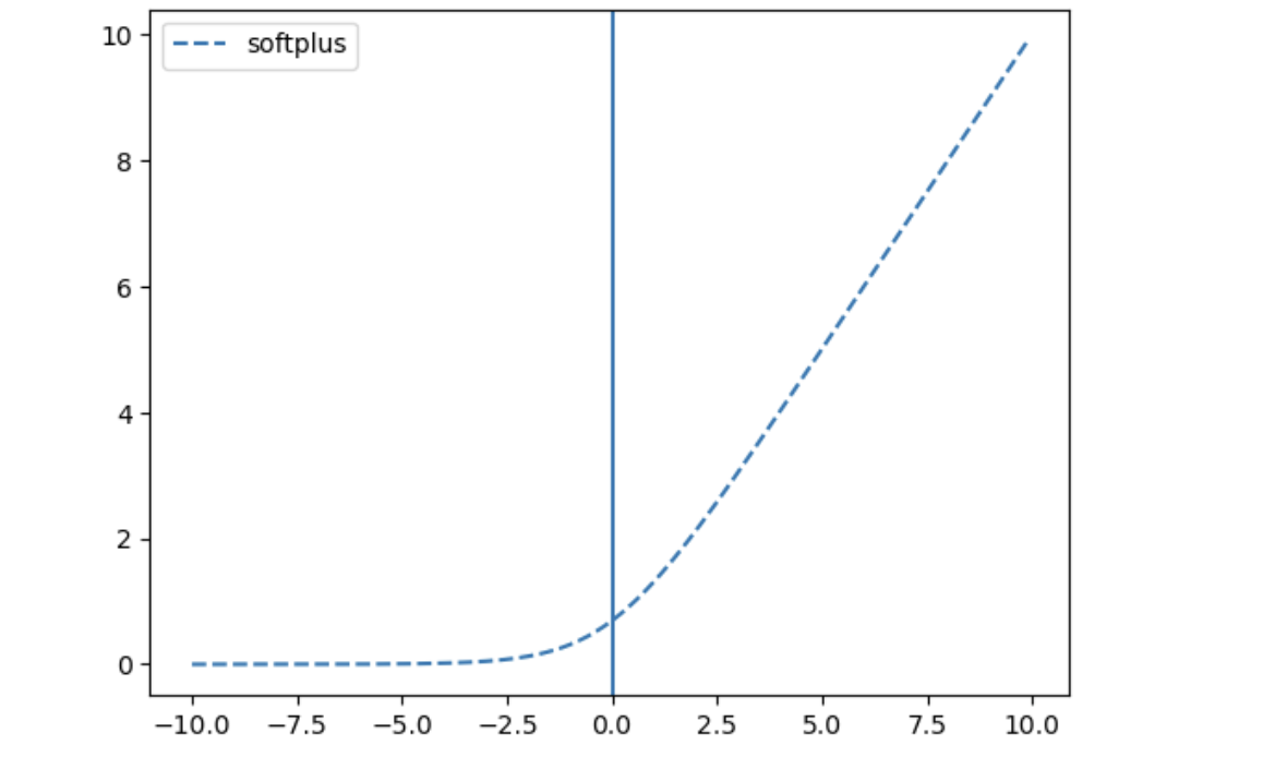

딥러닝 레이어

• 첫 번째 Dense 층은 128개의 노드를 가진다.
• 마지막층은 출력층
  - softmax
  • N개의 확률을 반환하고 반환된 값의 전체의 합은 1
  • 각 노드는 현재 이미지가 N개 클래스 중 하나에 속할 확율을 출력
  -Sigmoid
  • 둘 중 하나를 예측할 때 1개의 출력값을 출력함. 확률을 받아 임계값 기준으로 True, False로 나눔
• dropout(드롭아웃)
  : 층에 적용하면 훈련하는 동안 층의 출력 특성을 랜덤하게 끕니다. (즉, 0으로 만든다)
  - 훈련하는 동안 어떤 입력 샘플에 대해 [0.2, 0.5, 1.3, 0.8, 1.1] 백터를 출력하는 층이 있다고 가정
  - 드롭아웃을 적용하면 이 벡터에서 몇 개의 원소가 랜덤하게 0이 된다.
  [0.2, 0.5, 1.3, 0.8, 1.1] ➡️ [0, 0.5, 1.3, 0, 1.1]
  • 보통 0.2~0.5 사이를 사용

    입력데이터 수 구하기

 input_shape = X.shape[1]

input-hidden-output layers

 # 이진분류 ->sigmoid
 # 다중분류 ->softmax
 
 model = tf.keras.models.Sequential([
 	tk.keras.layers.Dense(units=128, input_shape=[input_shape]), 
    tf.keras.layers.Dense(128, activation='selu'),
  	tf.keras.layers.Dense(128, activation='selu'),
  	tf.keras.layers.Dense(128, activation='selu'),
  	tf.keras.layers.Dropout(0.2),
  	tf.keras.layers.Dense(1, activation='sigmoid')])

compile

• optimizer : 데이터와 손실함수를 바탕으로 모델의 업데이트 방법을 결정
• loss function : 훈련 하는 동안 모델의 오차를 측정한다. 모델의 학습이 올바른 방향으로 향하도록 이 함수를 최소화해야 한다.
  - 회귀 : MSE, MAE
  - 분류 :
  • 이진분류 : binary_crossentropy
  • 다중분류 : categorical_crossentropy(one-hot-encoding)
    sparse_categorical_crossentropy(ordinal_encoding)

 model.compile(optimizer='adam',
 				loss='binary_crossentropy', 
                metrics=['accuracy'])

summary

model.summary()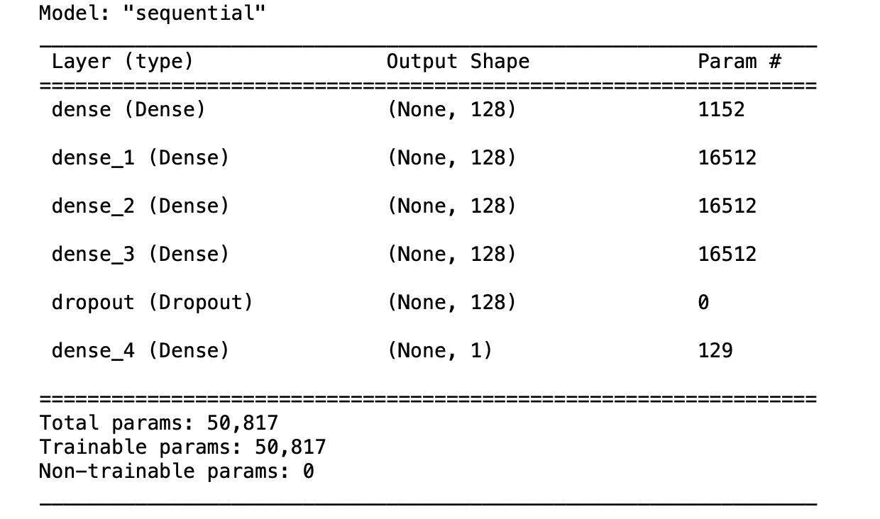

학습

• batch : 모델 학습에 한 번에 입력할 데이터셋
• epoch : 모델 학습 시 전체 데이터를 학습한 횟수
• step : (모델 학습의 경우) 하나의 배치를 학습한 횟수

EarlyStopping

class PrintDot(tf.keras.callbacks.Callback):
    def on_epoch_end(self, epoch, logs):
        if epoch % 100 == 0: print('')
        print('.', end='')

early_stop = tf.keras.callbacks.EarlyStopping(monitor='val_loss', patience=30)

학습

history = model.fit(X_train, y_train, epochs=1000, validation_split=0.2, callbacks=[early_stop, PrintDot()], verbose=0)

# 학습 결과의 history 값을 가져와서 비교하기 위해 데이터프레임으로 반환
```python
df_hist = pd.DataFrame(history.history)
df_hist.tail()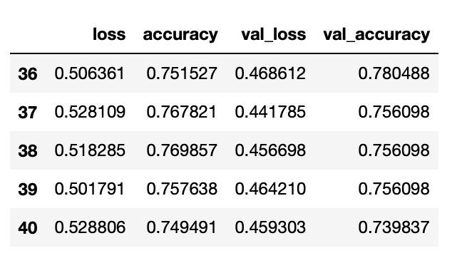

학습결과 시각화

df_hist[['loss', 'val_loss']].plot()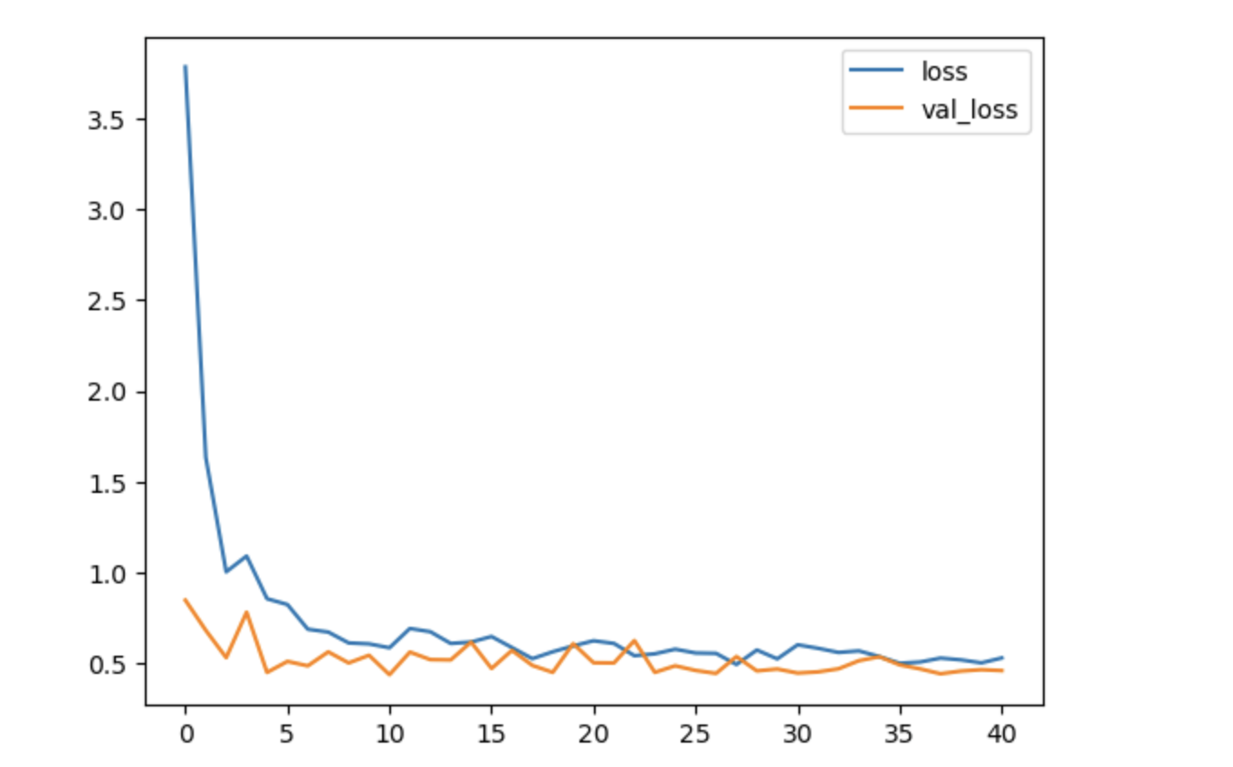

df_hist[['accuracy', 'val_accuracy']].plot()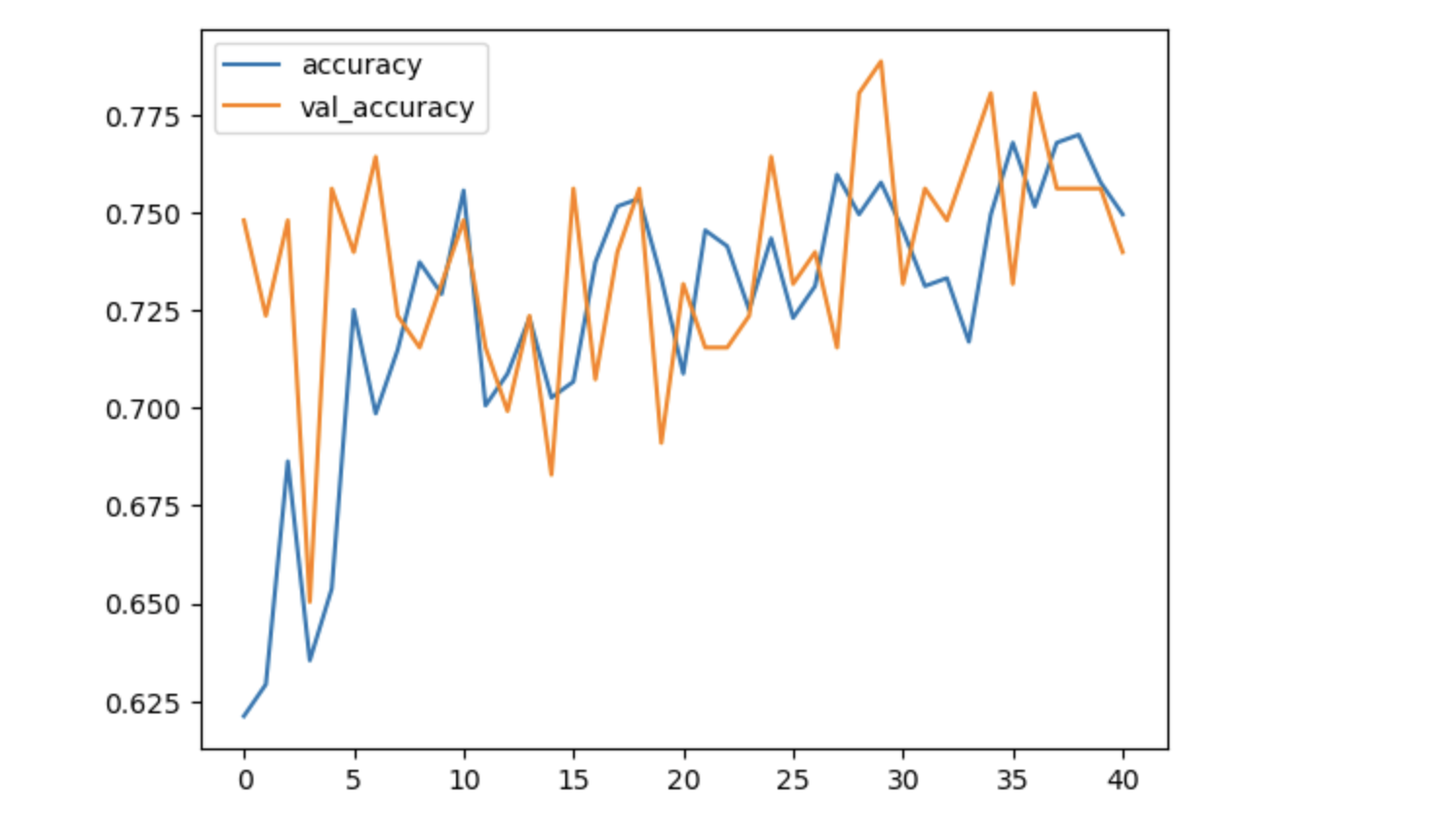

예측

• 예측값은 y_pred 변수에 할당 후 재사용
• binary -> 예측값이 각 row당 예측값 하나씩 나옴
• 여기에 나오는 확률값(sigmoid) 0~1 사이의 값을 갖는다
• 특정 임계값을 정해서 크고 작다를 통해 True, False 값으로 판단
• 임계값은 보통 0.5를 사용하지만 다른 값을 사용하기도 함

y_pred = model.predict(X_test)
y_pred.shape
>>>> (154, 1)

# 임계값(0.5)을 정해서 특정값 이상이면 True, 아니면 False로 변환해서 사용
# flatten() : 예측값을 1차원으로 변환

y_predict = (y_pred.flatten() > 0.5).astype(int)
y_predict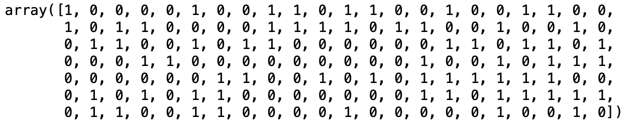

평가

test_loss, test_acc = model.evaluate(X_test, y_test)
test_loss, test_acc
>>>> loss: 0.6754 - accuracy: 0.7403

# 직접 정확도 구하기
(y_test == y_predict).mean()
>>>> 0.7402597402597403