PyTorch를 간단히 다루어본 적이 있는데, 앞으로의 연구에 익숙하게 활용하기 위해 PyTorch 내용을 정리해보려 한다.
대부분의 내용은 유튜브의 '모두를 위한 딥러닝 시즌2'를 참고하였다.
기본적인 딥러닝 내용과 파이썬 문법은 어느 정도 알고 있다고 가정하고, PyTorch 실습 내용 위주로 정리해두었다.
간단한 설명이 포함된 실습 자료는 Github를 참조하자.
1. ReLU (Rectified Linear Unit)
1) Problem of Sigmoid Function
Sigmoid function은 Vanish Gradient Problem이라는 큰 문제점이 존재한다.
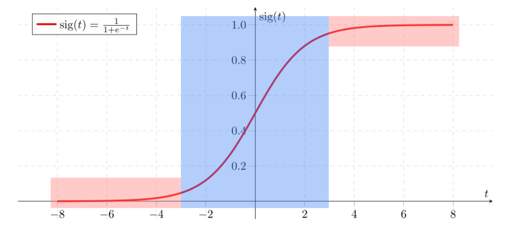
Backpropagation 과정에서 gradient를 구하여 곱하게 되는데, sigmoid 함수는 위와 같이 양쪽 끝 지점에서의 기울기가 매우 작으므로, layer가 깊을수록 그 기울기의 값이 0에 수렴해버린다.(vanishing, 즉 값의 영향이 사라져버리는 것이다.)
2) ReLU
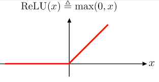
이를 해결하기 위해 제안된 Optimizer가 바로 Rectified Linear Unit이다.
먼저, ReLU 함수의 수식과 그래프 개형은 다음과 같다.
PyTorch에서의 함수는 다음과 같다.
x = torch.nn.relu(x)이외의 다양한 activation function을 사용할 수 있다.
x = torch.nn.sigmoid(x)
x = torch.nn.tanh(x)
x = torch.nn.leaky_relu(x, 0.01)
3) Optimizers in PyTorch
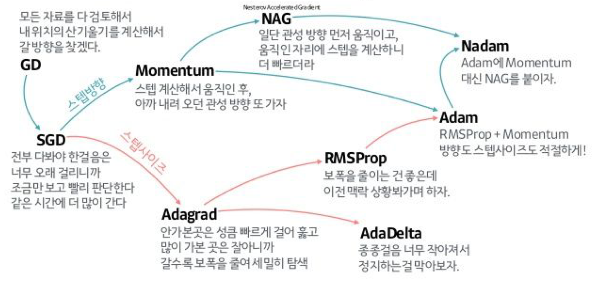
torch.nn 함수 내에서는 다음과 같은 다양한 optimizer를 제공한다.
torch.optim.SGD
torch.optim.Adadelta
torch.optim.Adagrad
torch.optim.Adam # 많이 사용!
torch.optim.SparseAdam
torch.optim.Adamax
torch.optim.ASGD
torch.optim.LBFGS
torch.optim.RMSprop # 많이 사용!
torch.optim.Rprop
각각의 자세한 원리는 여기서 다루지 않겠다.
대신, 다음 그림을 통해 개념적으로 여러 Optimizer를 파악할 수 있다.
2. Weight Initialization
인공지능 분야를 개척했다고 알려진 제프리 힌턴(Geoffrey Hinton) 교수는 weight initialization을 강조했다.
그 이유와 여러 초기화 방법을 알아보자.
1) Why Good Initialization?
먼저, 가중치 초기화가 왜 중요한지 알아보자.
지금까지 실습에서 항상 가중치를 무작위로 초기화하였다.
하지만, 다음 그림을 보자.
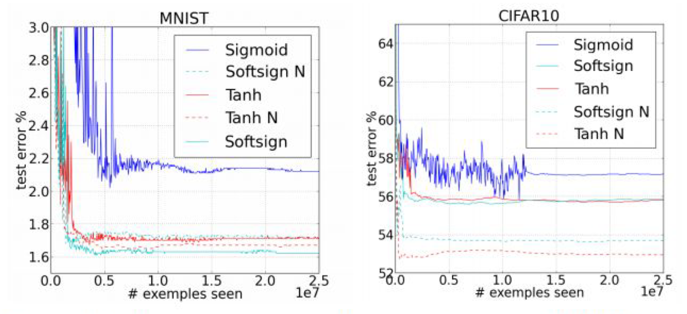
위 그림은 MNIST와 CIFAR10 데이터셋에 대한 error curve이다.
그래프의 색은 서로 다른 optimizer를 뜻하고, 실선과 점선은 weight initialization 방식에 따라 나뉜다.
한 눈에 보아도, 같은 색의 그래프에서 점선이 훨씬 더 좋은 성능을 보이는 것을 알 수 있다.
이때 N(점선)으로 표시된 것은, 무작위로 초기화하는 것이 아닌 Normalized Initialization을 뜻한다.
2) Weight Initialization Methods
그렇다면 어떻게 초기화하는 것이 현명한 방법일까?
일단, 모두 0으로 초기화하는 것은 안된다. 왜냐하면 gradient를 계산하는 과정에서 모두 0이면 학습이 진행되지 않기 때문이다.
Hinton 등은 2006년의 논문에서 Restricted Boltzmann Machine (RBM)을 이용하여 초기화하였을 때 Deep Neural Network의 성능이 훨씬 좋아졌다는 것을 보였다.
(1) Restricted Boltzmann Machine
Restricted라는 의미는 하나의 Layer 내의 노드 간에는 연결이 없다는 의미이다.
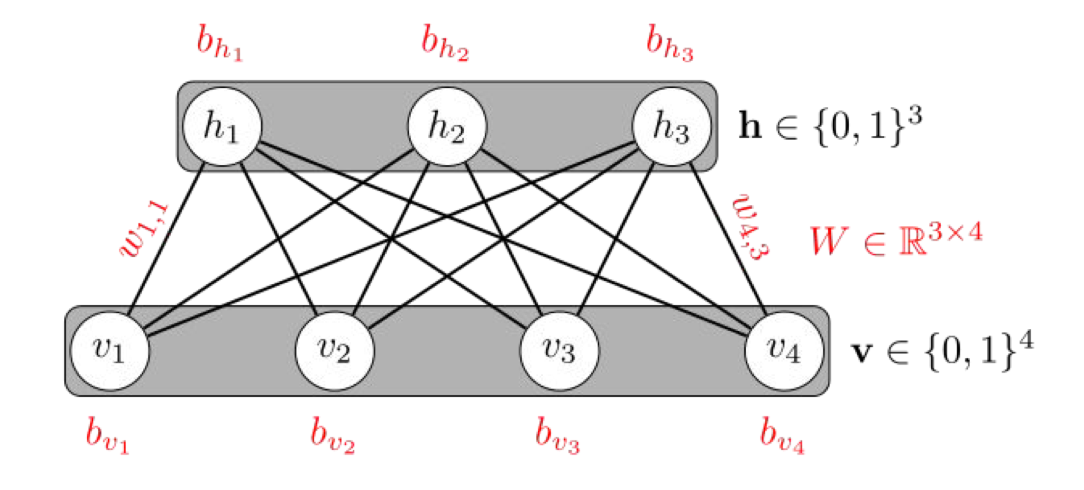
또한 위 사진과 같이 다른 layer 간의 노드끼리는 모두 연결이 된 형태이다.
이 Machine 내에서는 입력 x가 (v layer) 들어갔을 때, y (h layer)를 만들 수 있는 encoding 과정과, 반대로 y에서 x'으로 돌아가는 decoding 과정이 있다.
Hinton 교수는 이러한 RBM의 원리를 인접한 두 layer 간의 pre-training step에 적용하였다.
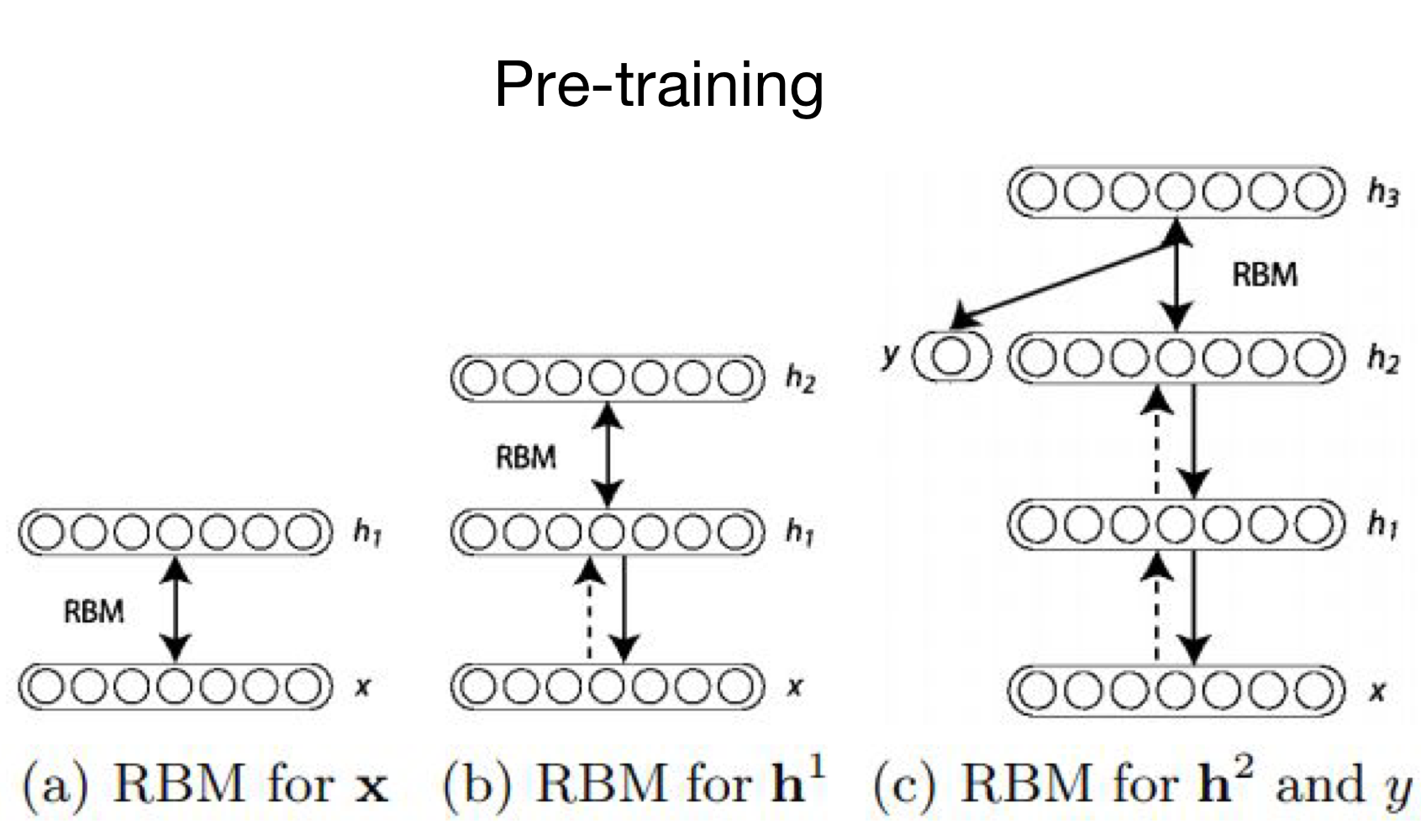
Pre-training은 다음의 과정을 거친다.
- (a)에서와 같이 두 개의 layer를 RBM으로 학습한다.
- (b)에서와 같이 와 간의 parameter(weight)는 고정시키고, layer와 새로운 layer를 RBM으로 학습한다.
- 위 과정을 마지막 layer까지 반복한다.
이를 이용하여 Fine-tuning의 과정을 거친다.
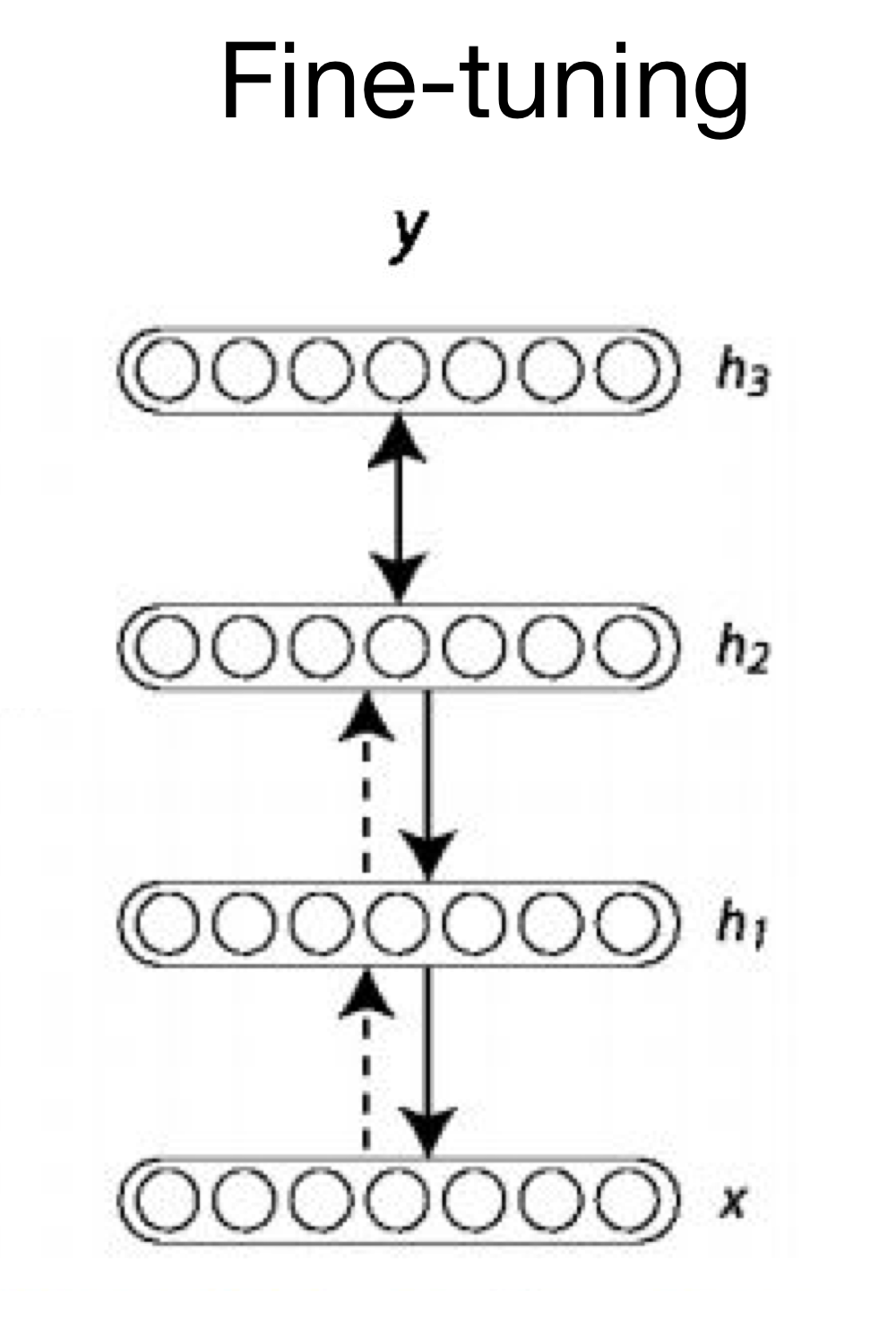
이미 RBM을 통해 초기화가 된 weight를 사용하여 y 및 loss를 구하여 backpropagation 등의 알고리즘에 따라 학습을 진행하는 것을 Fine-tuning이라 한다.
(2) Xavier Initialization / He Initialization
RBM을 이용한 initialization은 매우 복잡하지만, 시간이 지나면서 더 간단하고 좋은 성능을 보이는 initialization 알고리즘이 개발되었다.
먼저, Xaiver Initialization은 2010년에 고안된 알고리즘으로, 단순히 Normal distribution 또는 Uniform distribution으로 가중치를 초기화한다.
[Xavier Normal Initialization]
여기서 은 layer의 input node 개수를, 은 layer의 output node 개수를 말한다.
[Xavier Uniform Initialization]
He Initialization도 똑같이 표준분포와 균일분포를 통해 생성하는데, 수식에 약간의 차이가 있다.
[He Normal Initialization]
[He Uniform Initialization]
단순히 Xavier Initialization의 수식에서 output node 개수 term만 없앴다는 사실을 알 수 있다.
3) Xavier Initialization Implementation
xavier initialization 실습을 진행해보자.
Xavier Initialization 함수는 다음과 같이 간단하게 적용할 수 있다.
torch.nn.init.xavier_uniform_(layer.weight)다른 부분의 실습 설명은 이전 포스팅을 참고하자.
import torch
import torchvision.datasets as dsets
import torchvision.transforms as transforms
import random

# parameters
learning_rate = 0.001
training_epochs = 15
batch_size = 100

# MNIST dataset
mnist_train = dsets.MNIST(root='MNIST_data/',
                          train=True,
                          transform=transforms.ToTensor(),
                          download=True)
mnist_test = dsets.MNIST(root='MNIST_data/',
                        train=False,
                        transform=transforms.ToTensor(),
                        download=True)

# Dataset Loader
data_loader = torch.utils.data.DataLoader(dataset=mnist_train,
                                          batch_size=batch_size,
                                          shuffle=True,
                                          drop_last=True)

# nn layers
linear1 = torch.nn.Linear(784, 256, bias=True)
linear2 = torch.nn.Linear(256, 256, bias=True)
linear3 = torch.nn.Linear(256, 10, bias=True)
relu = torch.nn.ReLU()

# xavier initialization
torch.nn.init.xavier_uniform_(linear1.weight)
torch.nn.init.xavier_uniform_(linear2.weight)
torch.nn.init.xavier_uniform_(linear3.weight)

# model
model = torch.nn.Sequential(linear1, relu, linear2, relu, linear3)

# define cost & optimizer
criterion = torch.nn.CrossEntropyLoss() # softmax is internally computed.
optimizer = torch.optim.Adam(model.parameters(), lr=learning_rate)

total_batch = len(data_loader)
for epoch in range(training_epochs):
    avg_cost = 0

    for X, Y in data_loader:
        # reshape input image into [batch_size by 784]
        # label is not one-hot encoded
        X = X.view(-1, 28 * 28)

        optimizer.zero_grad()
        hypothesis = model(X)
        cost = criterion(hypothesis, Y)
        cost.backward()
        optimizer.step()

        avg_cost += cost / total_batch

    print('Epoch: ', '%04d' % (epoch + 1), 'cost: ', '{:.9f}'.format(avg_cost))

print('Learning finished')

# Test the model using test sets
with torch.no_grad():
    X_test = mnist_test.test_data.view(-1, 28 * 28).float()
    Y_test = mnist_test.test_labels

    prediction = model(X_test)
    correct_prediction = torch.argmax(prediction, 1) == Y_test
    accuracy = correct_prediction.float().mean()
    print('Accuracy: ', accuracy.item())

    # Get one and predict
    r = random.randint(0, len(mnist_test) - 1)
    X_single_data = mnist_test.test_data[r:r + 1].view(-1, 28 * 28).float()
    Y_single_data = mnist_test.test_labels[r:r + 1]

    print('Label: ', Y_single_data.item())
    single_prediction = model(X_single_data)
    print('Predcition: ', torch.argmax(single_prediction, 1).item())
Test 결과는 다음과 같다.
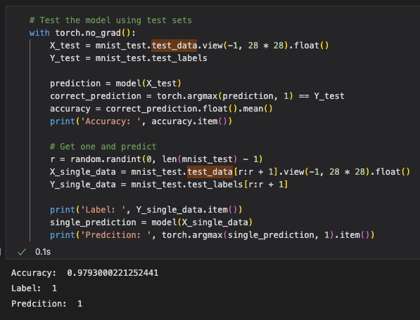
결과를 통해 weight 초기화 방법을 바꾸는 간단한 작업 하나로도 정확도를 꽤 향상시킬 수 있음을 알 수 있다.