PyTorch를 간단히 다루어본 적이 있는데, 앞으로의 연구에 익숙하게 활용하기 위해 PyTorch 내용을 정리해보려 한다.
대부분의 내용은 유튜브의 '모두를 위한 딥러닝 시즌2'를 참고하였다.
기본적인 딥러닝 내용과 파이썬 문법은 어느 정도 알고 있다고 가정하고, PyTorch 실습 내용 위주로 정리해두었다.
간단한 설명이 포함된 실습 자료는 Github를 참조하자.
1. Perceptron
Perceptron은 인공 신경망의 기본 unit이다.
인공 신경망은 뇌의 '뉴런'의 동작 방식을 본따 만들었다.
뉴런 각각의 동작 방식은 매우 간단하다.
입력 신호를 받아 그 신호 값이 threshold를 넘게 되면 신호를 전파하고, 다음 뉴런으로 그 신호를 전해주게 된다.
이러한 인공신경망 중의 하나인 perceptron에 대해 알아보자.
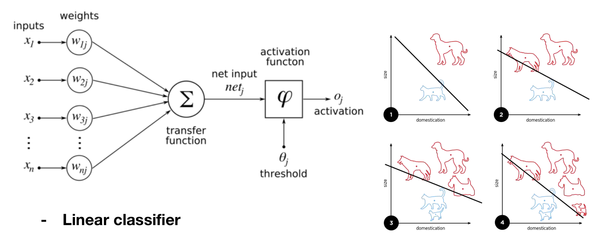
Perceptron은 입력 에 가중치 를 곱한 후 bias 와 더해지고, activation function을 거쳐 output을 낸다.
초창기 Perceptron은 Linear Classifier로 사용되었다.
1) AND, OR Problem
1950년대에 Perceptron이 개발되었는데, 이 때에는 AND, OR 문제를 해결하기 위해 사용되었다.
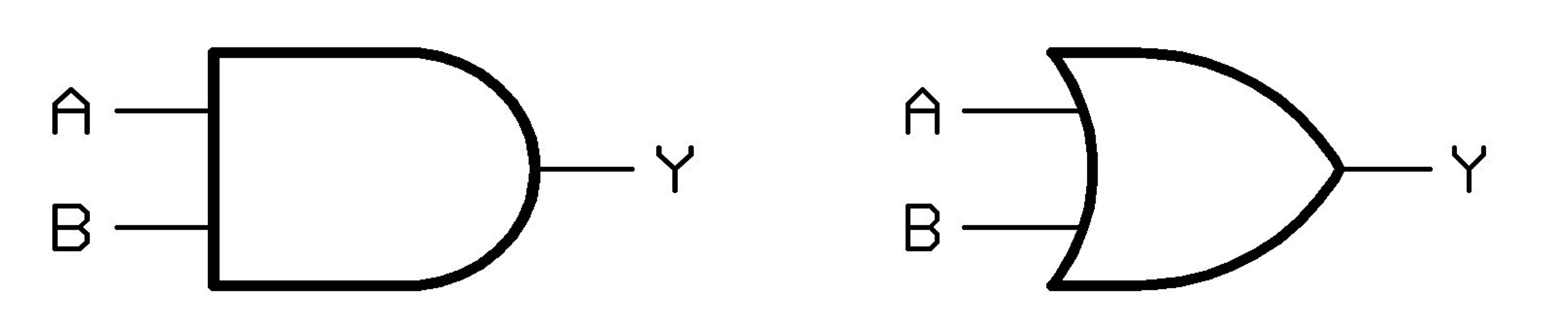
[AND Gate]
| A | B | result |
|---|---|---|
| 0 | 0 | 0 |
| 0 | 1 | 0 |
| 1 | 0 | 0 |
| 1 | 1 | 1 |
[OR Gate]
| A | B | result |
|---|---|---|
| 0 | 0 | 0 |
| 0 | 1 | 1 |
| 1 | 0 | 1 |
| 1 | 1 | 1 |
아래 그림을 보면 Perceptron을 통해 AND, OR 문제를 잘 해결할 수 있음을 알 수 있다.
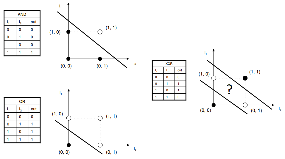
Linear Classifier로 이러한 문제를 해결하면서, 인공신경망은 크게 주목받기 시작했다.
2) XOR Problem
하지만, 민스키가 Perceptron 구조로는 XOR 문제를 해결할 수 없다는 사실을 증명하였다.
하나의 Linear Classifier로는 위 그림처럼 XOR 문제를 해결할 수 없다는 결론을 얻은 것이다.
XOR 문제는 다음과 같다.
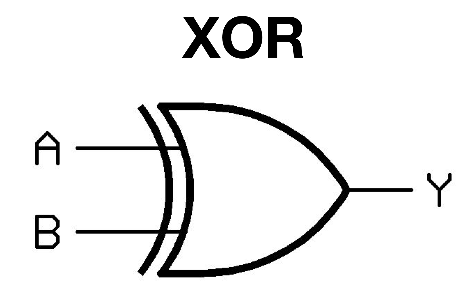
[XOR Gate]
| A | B | result |
|---|---|---|
| 0 | 0 | 0 |
| 0 | 1 | 1 |
| 1 | 0 | 1 |
| 1 | 1 | 0 |
이로 인해 인공신경망 분야는 암흑기에 빠지게 된다.
XOR Implementation
code로 XOR Problem을 Perceptron으로 해결해보자.
import torch

X = torch.FloatTensor([[0, 0], [0, 1], [1, 0], [1, 1]])
Y = torch.FloatTensor([[0], [1], [1], [0]])

# nn layers
linear = torch.nn.Linear(2, 1, bias=True) # FC Layer
sigmoid = torch.nn.Sigmoid() # activation function
model = torch.nn.Sequential(linear, sigmoid)

# define cost & optimizer
criterion = torch.nn.BCELoss() # binary cross entropy loss (0, 1 분류)
optimizer = torch.optim.SGD(model.parameters(), lr=1)

for step in range(10001):
    optimizer.zero_grad()
    hypothesis = model(X)
    # cost function
    cost = criterion(hypothesis, Y)
    cost.backward()
    optimizer.step()
    if step % 1000 == 0:
        print(step, cost.item())
결과는 다음과 같다.
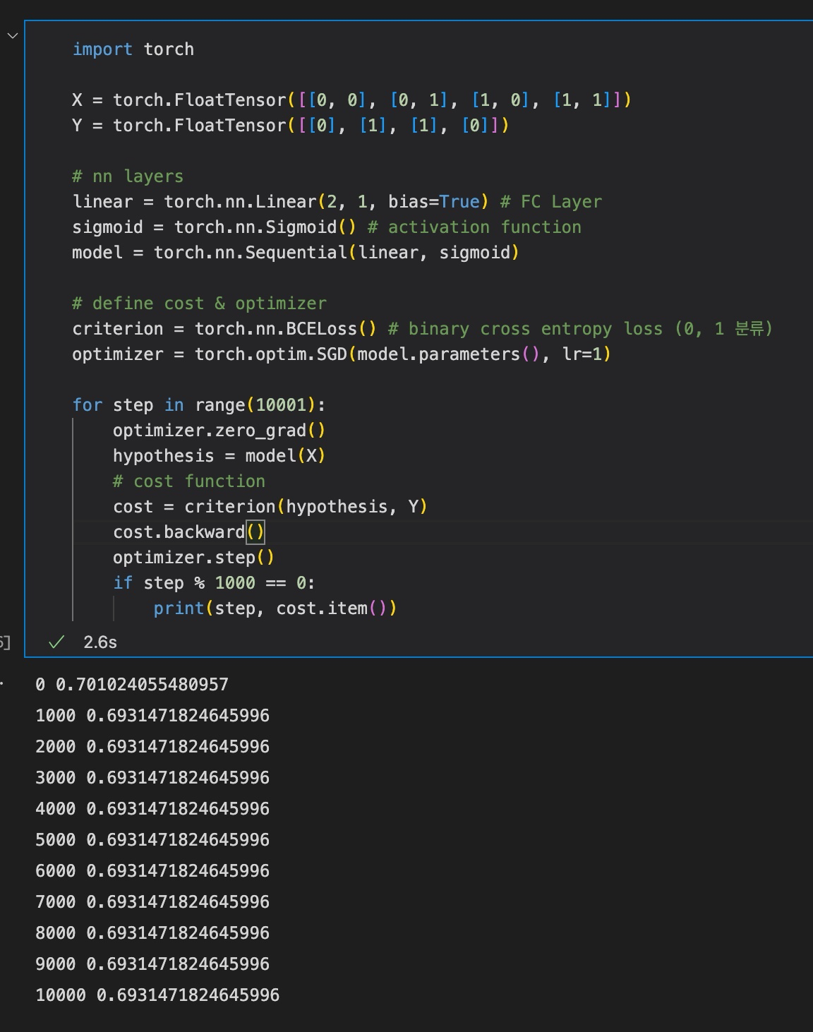
결과를 살펴보면, 약 200 step 이후부터는 loss가 줄지 않는다. 즉, 학습이 제대로 진행되지 않는다.
test를 진행하면 다음과 같은 결과를 얻을 수 있다.
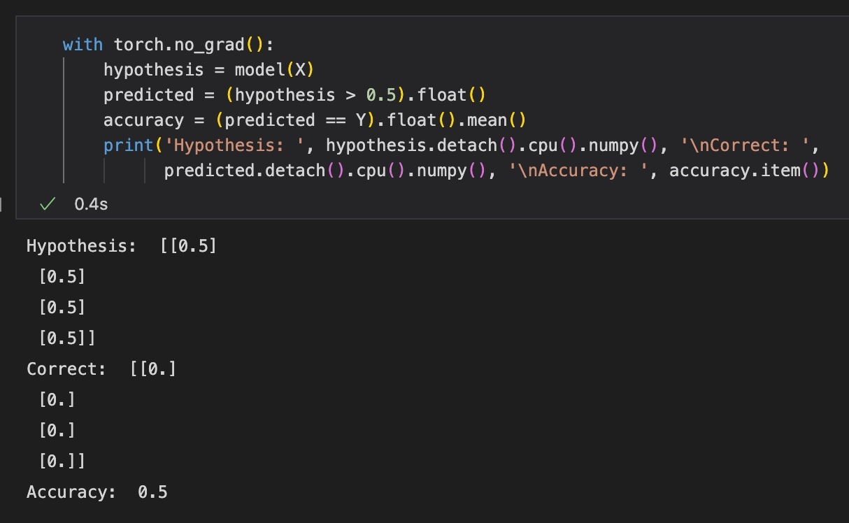
학습이 끝난 후에 각 x에 대한 결과값을 보면, perceptron 모델이 모든 값을 0.5로 예측하고 있음을 알 수 있다. 실제로는 [0, 0, 0, 0]을 나타내므로 정확도도 50%에서 더 나아지지 않는다.
2. Multi Layer Perceptron (MLP)
그러면 XOR 문제를 해결하려면 어떻게 해야할까?
Perceptron은 단순히 linear classifier이지만, XOR 분류 문제에서는 고차원의 분류기를 사용해야 할 것이다.
1) Multi Layer Perceptron
다음 사진을 보자.
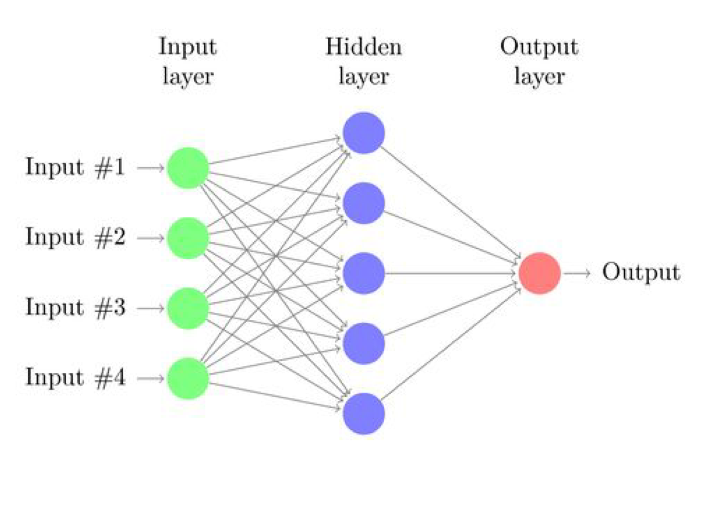
위의 XOR 문제 그림에서, 하나의 선으로는 구분이 불가능했다. 하지만, 선 하나를 더 긋는다면 (Perceptron 두 개를 사용한 모델) 해결이 가능해진다.
하지만 당시에는 여러 퍼셉트론을 학습할 방법이 없었고, 그렇게 인공신경망 분야는 암흑기에 빠졌다.
2) Backpropagation
Backpropagation 알고리즘은 loss(error)를 output단에서부터 input단으로까지 전파시키며 weight를 업데이트하는 알고리즘이다.
이는 현재에도 사용되는 알고리즘이며, 이 때부터 MLP를 학습할 수 있게 되었다.
Backpropagation Implementation
Backpropagation 알고리즘 실습을 진행해보자.
먼저, 라이브러리를 import하고, 데이터와 라벨을 생성한다.
import torch

X = torch.FloatTensor([[0, 0], [0, 1], [1, 0], [1, 1]])
Y = torch.FloatTensor([[0], [1], [1], [0]])
다음으로, 3가지 인공신경망 layer를 생성해준다. backpropagation 과정을 자세히 알아보기 위해 weight, bias를 따로 선언해주었고, sigmoid 함수와 sigmoid 함수의 미분까지 함수로 구현해주었다.
w1 = torch.Tensor(2, 2)
b1 = torch.Tensor(2)
w2 = torch.Tensor(2, 1)
b2 = torch.Tensor(1)

def sigmoid(x):
	# sigmoid function
    return 1.0 / (1.0 + torch.exp(-x))

def sigmoid_prime(x):
	# derivative of the sigmoid function
    return sigmoid(x) * (1 - sigmoid(x))
실제 구현 시에는 nn.Linear 함수를 사용하면 다음과 같이 간단히 표현 가능하다.
# nn layers
linear1 = torch.nn.Linear(2, 2, bias=True)
linear2 = torch.nn.Linear(2, 1, bias=True)
sigmoid = torch.nn.Sigmoid()
sigmoid는 activation 함수이므로 각 linear layer 이후에 한 번씩 붙고, linear1은 입력 2개를 받아 출력으로 2개의 값을, linear2는 입력 2개를 받아 출력으로 하나의 값을 내는 layer이다.
즉, 총 2개의 layer를 갖는 Multi Layer Perceptron이다.
여기서 layer를 추가하여 더 깊은(deep) MLP를 만들 수 있으며, 입출력 노드 개수를 늘림으로써 더 넓은(wide) MLP를 만들 수 있다.
다음으로 cost function과 optimizer를 선언한다.
# define cost & optimizer
criterion = torch.nn.BCELoss()
optimizer = torch.optim.SGD(model.parameters(), lr=1)
학습은 다음과 같이 진행된다.
먼저 backpropagation 과정을 자세히 나타낸 코드를 보자.
for epoch in range(10001):
	# forward propagation (cost 계산 과정)
    l1 = torch.add(torch.matmul(X, w1), b1)
    a1 = sigmoid(l1)
    l2 = torch.add(torch.matmul(a1, w2), b2)
    Y_pred = sigmoid(l2)

    cost = -torch.mean(Y * torch.log(Y_pred) + (1 - Y) * torch.log(1 - Y_pred)) # binary cross entropy loss
    # back propagation (chain rule)
    # Loss derivative
    d_Y_pred = (Y_pred - Y) / (Y_pred * (1.0 - Y_pred) + 1e-7) # 0으로 나누지 않도록 1e-7 더함
    # Layer 2
    d_l2 = d_Y_pred * sigmoid_prime(l2)
    d_b2 = d_l2
    d_w2 = torch.matmul(torch.transpose(a1, 0, 1), d_b2)

    # Layer 1
    d_a1 = torch.matmul(d_b2, torch.transpose(w2, 0, 1))
    d_l1 = d_a1 * sigmoid_prime(l1)
    d_b1 = d_l1
    d_w1 = torch.matmul(torch.transpose(X, 0, 1), d_b1))

    # Weight update
    w1 = w1 - learning_rate * d_w1
    b1 = b1 - learning_rate * torch.mean(d_b1, 0)
    w2 = w2 - learning_rate * d_w2
    b2 = b2 - learning_rate * torch.mean(d_b2, 0)

    if epoch % 100 == 0:
    	print(epoch, cost.item())
Backpropagation 부분의 전체적인 코드 흐름을 살펴보면, error가 derivative 함수(sigmoid_prime)를 따라 output 방향에서 input 방향으로 전파됨을 알 수 있다.
또한, weight update가 gradient descent에 따라 이루어짐을 살펴볼 수 있다.
PyTorch에서는 backward(), step()함수로 위와 같은 긴 과정을 간단히 구현할 수 있다.
for epoch in range(10001):
optimizer.zero_grad()
hypothesis = model(X)
# cost function
cost = criterion(hypothesis, Y)
cost.backward()
optimizer.step()
if epoch % 1000 == 0:
print('Epoch: {:4d} \\ Cost: {:.4f}'.format(
epoch, cost.item()
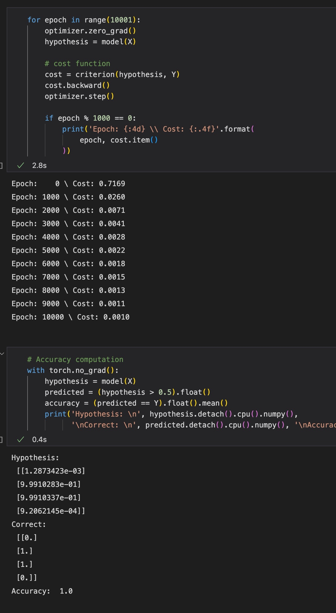
))학습된 모델을 Test한다.
# Accuracy computation
with torch.no_grad():
    hypothesis = model(X)
    predicted = (hypothesis > 0.5).float()
    accuracy = (predicted == Y).float().mean()
    print('Hypothesis: \n', hypothesis.detach().cpu().numpy(),
          '\nCorrect: \n', predicted.detach().cpu().numpy(), '\nAccuracy: ', accuracy.item())
최종 결과는 다음과 같다

좋은 자료 감사합니다.