Day 1

강의 듣기 - 딥러닝 기본, 최적화, 데이터 시각화

What make you a good deep learner

• Implementation Skills
• Math Skills (Linaer Algebra, Probability)
• Knowing a lot of recent Papers

Key Components of Deep Learning

• The data that the model can learn from (cat / dog, bounding box, etc...)
• The model how to transform the data (AlexNet, ResNet, etc ...)
• The loss function that quantifies the badness of the model (Cross Entropy, MSE, etc ...)
• The algorithm to adfust the parameters to minimize the loss (Adam, SGD, etc ...)

Historical Review

• 2012 - AlexNet : Conv Net, 딥러닝을 이용하여 ImageNet에서 1등을 함. 이 이후에는 딥러닝을 이용하지 않은 방법이 1등을 한 적이 없음.
• 2013 - DQN : 알파고의 강화학습의 기반이 된 모델
• 2014 - Encoder/Decoder, Adam
• 2015 - Gan, ResNet
• 2017 - Transformer
• 2018 - Bert : Fine-tuned 된 Language Model
• 2019 - Big Language Models (GPT-X)
• 2020 - Self-Supervised Learning
  (ex. SimCLR : a simple framework for contrastive learning of visual representations)

Neural Networks

• Neural Networks are function approximators that stack affine transformations followed by nonlinear transformations.

Multi Layer Perceptron

• Matrix Multiplication은 선형 변환. Deep Learning을 하기 위해 여러 개의 Matrix를 겹쳐봐야 그것은 또 하나의 Matrix, 즉 선형 변환이다. 그렇기 때문에 Matrix 사이에 Non linear function (=activation function)을 넣어 MLP를 구성함.

Optimization

• Generalization : How well the learned model will behave on unseen data
• Under-fitting vs Over fitting : 아예 학습이 되지 않은 것 vs 학습 데이터만 잘 맞추고, 다른 데이터는 잘 못 맞추는 것
• Cross-validation : model validation technique for assessing how the model will generalize to an independent (test) data set.
• Bias and Variance : 탄착군 형성 = low variance = 출력이 얼마나 일관성 있게 나오는가 / bias : 평균적으로 target과 비슷한가?
• Bias and Variance Tradeoff : $cost = bias^2 + variacne + noise$
• Bootstrapping : any test or metric that uses random sampling with replacement. => 학습 데이터의 subset들을 다양하게 이용하여 여러 모델, 메트릭을 만들어 uncertainty를 확인
• Bagging : Bootstrapping aggregating / Multiple models are being trained with bootstrapping.
• Boosting : It focuses on those specific training samples that are hard to classify. A strong model is built by combining weak learners in sequence where each learner learns from the mistakes of the previous weak learner.

Gradinet Descent Methods

• Stochastic Gradient Descent
• Mini-batch Gradient Descent
• Batch Gradient Descent
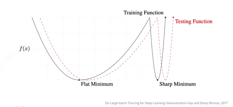
• Large Batch Size -> Sharp Minimizer (=generalization performance 가 나쁨)
• Small Batch Size -> Flat Minimizer (=generalization performance 가 좋음)
  

Boostcamp AI Tech 강의안에서 발췌함

Advanced Gradient Descent Methods

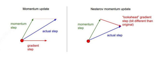
• (original) Gradient Descent : $W_{t+1}\leftarrow W_t -\eta g_t$
• Momentum : $\alpha_{t+1} \leftarrow \beta \alpha_t + g_t$, $W_{t+1} \leftarrow W_t - \eta \alpha_{t+1}$
• Nesterov Accelerated Gradient (NAG) : $\alpha_{t+1} \leftarrow \beta \alpha_t + \nabla \mathcal{L}(W_t - \eta \beta \alpha_t)$, $W_{t+1} \leftarrow W_t - \eta \alpha_{t+1}$
  $\nabla \mathcal{L}(W_t - \eta \beta \alpha_t)$ : Lookahead gradient - Local Minima에 좀 더 빠르게 도달
  

Boostcamp AI Tech 강의안에서 발췌함

• Adagrad : adpats the learning rate, performing larger updates for infrequent and smaller updates for frequent parameters.
  $W_{t+1} = W_t - \frac{\eta}{\sqrt{G_t + \epsilon}}g_t$
• Adadelta : extends Adagrad to reduce its monotonically decreasing the learning rate by restricting the accumulation window. $G_t$가 $t$가 늘어남에 따라 계속 증가하는 것을 $t$를 제한함으로써 방지함. Learning rate가 없음.
  $G_t = \gamma G_{t-1} + (1-\gamma)g_t^2$,
  $W_{t+1} = W_t - \frac{\sqrt{H_{t-1} + \epsilon}}{\sqrt{G_t+\epsilon}}g_t$,
  $H_t=\gamma H_{t-1}+(1-\gamma)(\triangle W_t)^2$
• RMSprop : unpublished, adaptive learning rate method proposed by Geoff Hinton in his lecture.
  $G_t = \gamma G_{t-1} + (1-\gamma)g_t^2$,
  $W_{t+1} = W_t - \frac{\eta}{\sqrt{G_t+\epsilon}}g_t$
• Adam : leverages both past gradients and squared gradients.
  momentum : $m_t = \beta_1m_{t-1}+(1-\beta_1)g_t$
  gradient squares = $v_t = \beta_2v_{t-1}+(1-\beta_2)g_t^2$,
  $W_{t+1}=W_t-\frac{\eta}{\sqrt{v_t+\epsilon}}\frac{\sqrt{1-\beta_2^t}}{1-\beta_1^t}m_t$

Regularization

• Early Stopping : Valid Error가 가장 낮을 때 stop.
• Parameter Norm Penalty : Adds Smoothness to the function space.
  $\text{total cost} = \text{loss}(\mathcal{D};W) + \frac{\alpha}{2}\|W\|_2^2$
• Data Augmentation : More data are always welcomed.
• Noise Robustness : Add random noises inputs or weights.
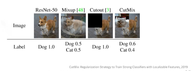
• Label Smoothing : Mix-up contructs augmented training examples by mixing both input and output of two randomly selected training data
  ex. CutMix constructs augmented training examples by mixing inputs with cut and paste and outputs with soft labels of two randomly selected training data.
  

Boostcamp AI Tech 강의안에서 발췌함

• Dropout : In each forward pass, randomly set some neurons to zero.
• Batch Normalization : compute the empirical mean and variance independently for each dimension (layers) and normalize. 각각의 layer의 값들을 정규화 시키고자 하는 것. 논문 曰 internal covariance shift (= feature) 를 줄여 더 잘 학습시키게 한다. 이후의 논문들은 이를 부정하기도 하지만, 일반적으로 layer를 깊게 쌓으면 성능이 좋아지긴 함.

데이터 시각화란

• 데이터를 그래픽 요소로 매핑하여 시각적으로 표현하는 것
• 시각화는 다양한 요소가 포함된 Task
  - 목적, 독자, 데이터, 스토리, 방법, 디자인

"데이터" 시각화

• 정형 데이터 : 테이블 형태.csv, tsv 파일로 제공되며, row가 데이터 1개. column은 attribute.
  통계적 특성과 feature 사이 관계 / 데이터 간 관계 / 데이터 간 비교
• 시계열 데이터 : 시간 흐름에 따른 데이터. 기온, 주가 (정형 데이터), 음성, 비디오 (비정형 데이터)
  추세 / 계절성 / 주기성
• 지리/지도 데이터 : 지도 정보와 정보 간의 조화가 중요함. 지도 정보를 단순화 시키는 경우도 존재
  거리 / 경로 / 분포 등 다양한 실사용
• 관계 데이터 : 객체와 객체 간의 관계를 시각화. 객체는 node로 관계는 link로 표현. 크기, 색, 수 등으로 객체와 관계의 가중치를 표현하고, 휴리스틱하게 노드 배치를 구성함.
• 계층적 데이터 : 관계 중 포함관계가 분명한 데이터. 네트워크 시각화로도 표현 가능. Tree, Treemap, Sunburst 등이 대표적

시각화 이해하기

• 마크 (Mark) : 점, 선, 면으로 이루어진 데이터 시각화
• 채널 (Channel) : 각 마크를 변경할 수 있는 요소들 (색, 위치, 모양, 기울기, 부피 등)
• 전주의적 속성 (Pre-attentive Attribute) : 주의를 주지 않아도 인지하게 되는 요소. 단, 동시에 사용하면 인지하기 어려움. 적절하게 사용해야 시각적 분리(visual pop-out)가 가능함.

코드로 이해하기 (basic)

import matplotlib.pyplot as plt

# subplot 객체 (ax) 생성하기
fig = plt.figure(figsize = (12, 8)) # figsize로 plot 비율 조정
ax1 = fig.add_subplot(121) # (1, 2, 1)과 동일
ax2 = fig.add_subplot(122) # (1, 2, 2)와 동일

# subplot 객체에 그리기
x1 = [1, 2, 3]
x2 = [3, 2, 1]
ax1.plot(x1)
ax2.plot(x2)
plt.show()

# color 사용하기
ax1.plot([1, 1, 1], color = 'r')		# 약어
ax1.plot([1, 1, 1], color = 'red')		# color name
ax1.plot([1, 1, 1], color = '#000000')	# hex code

# 범례 사용하기
ax1.plot([1, 1, 1], label = '1')
ax1.legend()

# 제목 생성하기
ax1.set_title('Basic Plot')
print(ax1.get_title()) >>> 'Basic Plot'

# 축에 이름 붙이기
ax1.plot([1, 1, 1], label = '1')
ax1.set_xticks([0, 1, 2]) > x축이 0, 1, 2로 표현
ax1.set_xticklabels(['zero', 'one', 'two']) 
> xticks로 정해주었던 0,1,2가 zero, one, two로 바뀜

# plot 안에 text 넣기
ax1.text(x = 1, y = 2, s = 'This is Text')
> x=1, y=2 의 위치에 This is Text가 생성됨
> ax.annotate(text = 'This is Text', xy = (1, 2)) 와 동일

# annotate 추가 기능
ax1.annotate(text = 'This is Annotate', xy = (1, 2),
			 xytext = (1, 2, 2.2),
             arrowprops = dict(facecolor = 'black'))
> 화살표도 plot에 넣을 수 있음

Day2

강의 듣기 - CNN

Convolution

• Continuous Convolution : $(f*g)(t) = \int{f(\tau)g(t-\tau)d\tau}=\int f(t-\tau)g(t)d\tau$
• Discrete Convolution : $(f*g)(t) = \sum_{i=-\infty}^{\infty}{f(i)g(t-i)}=\sum_{i=-\infty}^{\infty} f(t-i)g(t)$
  -2D Image Convolution:
  $(I*K)(i, j)=\sum_{m}\sum_{n}I(m,n)K(i-m,j-n)=\sum_{m}\sum_{n}I(i-m, i-n)K(m, n)$

Convolutional Neural Neworks

• CNN consists of convolution layer, pooling layer, fully connected layer
• Convolution and Pooling Layers : feature extraction
• Fully Connected Layer : Decision Making -> too many parameters

1*1 convolution

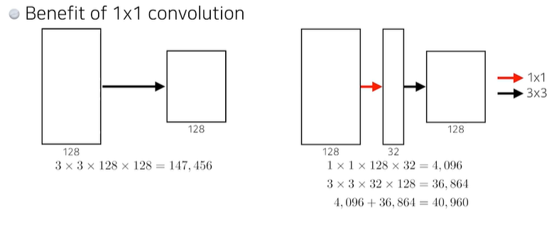
• parameter를 줄이기 위해 사용됨.
• 128*256*256 -> 32*256*256 으로 줄이는 과정에서
  • 1*1 convolution을 사용한다면 parameter의 수는 1*1*128*32 = 4096
  • fc layer를 사용한다면 flatten 후 각 뉴런마다 모든 뉴런에 대해 계산을 하므로 parameter 수가 매우 많아짐.

Modern CNN - AlexNet

• 11*11*3 filter(=kernel)을 사용함.
• 5개의 convolution layer, 3개의 dense layer
• ReLU를 사용함
• 2 GPU 사용
• Local Response Nomalization, Overlapping Pooling
• Data Augmentation
• Dropout

Modern CNN - VGGNet

• 3*3 filter
• 1*1 convolution
• Dropout
• 16 layers, 19 layers

Modern CNN - GoogLeNet

• 22 layers
• Network in Network
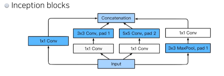
• Inception blocks
  • reduce the number of parameter (1*1 convolution)
  • 1*1 convolution can be seen as channel-wise dimension reduction
    

Boostcamp AI Tech 강의안에서 발췌함

Boostcamp AI Tech 강의안에서 발췌함

Modern CNN - ResNet

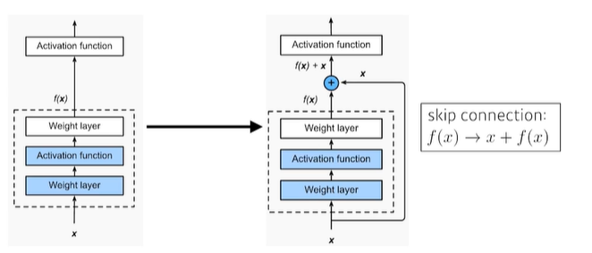
• Deeper neural networks are hard to train
  • Overfitting is usually caused by an excessive number of parameters
• Add an identity map (skip connection)
  

Boostcamp AI Tech 강의안에서 발췌함

• Batch normalization after convolutions
• Bottleneck architecture (using 1*1 filter)

Modern CNN - DenseNet

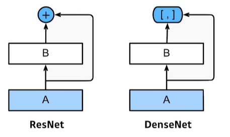
• DeseNet uses concatenation instead of addition
  

Boostcamp AI Tech 강의안에서 발췌함

• concatenation 하면 channel이 커짐. 그렇기 때문에 중간에 1*1 convolution을 통해 channel을 압축
• Dense Block
  • Each layer concatenates the feature maps of all preceding layers
  • The number of channels increases geometrically
• Transition Block
  • BatchNorm -> 1*1 conv -> 2*2 AvgPooling
  • Dimension reduction
    

Boostcamp AI Tech 강의안에서 발췌함

Semantic Segmentation

• 이미지를 보고 픽셀별로 classification 하는 것
• 자율주행에서 활용 가능
• Fully Convolutional Network
  • Trnasforming fully connected layers into convolution layers enbales a classification net to output a heat map
  • Upsampling을 해야 함. convolution layer를 거쳐 작아진 image feature를 다시 원 상태로 복구시켜야 함 -> Deconvolution
  • Deconvolution은 완벽한 convolution의 역연산이 아님.

Detection

• R-CNN (Regional CNN)
  • 이미지를 무작위로 추출한 후, CNN 돌린 다음, SVM으로 분류.
  • 문제점 : 추출한 이미지를 모두 CNN에 돌리기 때문에 너무 많은 연산이 필요함.
• SPPNet : R-CNN의 많은 연산량을 보완함. 이미지를 CNN에 돌린 후, bounding box에 맞는 tensor만 뽑아오자
• Fast R-CNN : SPPNet과 거의 비슷함. 뒷단의 neural network를 통해 bounding box를 어떻게 움직이면 좋을지 예측하는 모델이 추가됨.
• Faster R-CNN : bounding box를 뽑아낼 때 무작위로 뽑지 말고 그것도 알고리즘으로 만들자(Region Proposal Network). 그 후에 Fast R-CNN.
• YOLO : It simultaneously predicts multiple bounding boxes and class probabilities. No explicit bounding box sampling (compared with Faster R-CNN). 즉, bounding box를 추출하는 과정이 없음.
  • image가 들어오면 image를 S*S gird로 나누게 됨
    • 만약 물체의 중앙이 그 grid 셀 안에 들어있다면 그 grid 셀은 detection의 원인이 됨.
  • 각각의 셀은 B개의 bounding box를 예측함. 각각의 셀은 어떤 클래스인지 예측함.
    • Each bounding box predicts
      • box refinement(x, y, h, w)
      • confidence (of objectness)
  • 그래서 결과적으로 S*S*(B*5+C) 사이즈의 텐서가 나옴.
    • S*S : Number of cells of the grid
    • B*5 : B bounding boxes with offsets (x, y, w, h) and confidence
    • C : Number of classes

Sequential Models

• 입력의 길이, dimension이 가변적이다.
• Naive Seqeunce Model
  • Autogregressive model, Markov model : 과거 특정 몇 개의 데이터만 사용하겠다..!
  • Latent Autoregressive model : 과거의 데이터를 요약하는 hidden state를 추가해서 사용..!

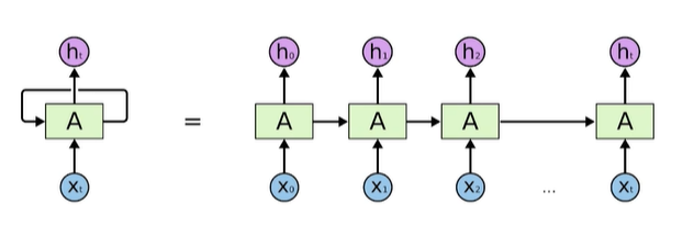
Vanilla RNN (Recurrent Neural Network)

• Short term dependencies : 옛날의 데이터가 전달되지 않을 수 있음..
  $h_1 = \phi(W^Th_0 + U^Tx_1)$
  $h_2 = \phi(W^T(\phi(W^Th_0 + U^Tx_1)) + U^Tx_2)$
  $h_3 = \phi(W^T(\phi(W^T(\phi(W^Th_0 + U^Tx_1)) + U^Tx_2)) + U^Tx_3)$
  $h_4 = \phi(W^T(\phi(W^T(\phi(W^T(\phi(W^Th_0 + U^Tx_1)) + U^Tx_2)) + U^Tx_3)) + U^Tx_4)$
  $\phi$, $W^T$가 계속 곱해지면서 gradient vanishing, expliding이 발생할 수 있음. (Sigmoid or TanH면 vanishing, ReLU를 쓴다면 exploiding 발생 가능)
  

Boostcamp AI Tech 강의안에서 발췌함

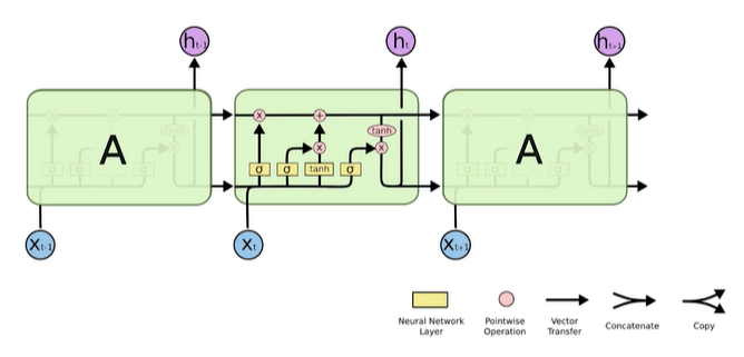
LSTM (Long Short Term Memory)

• Core idea - Cell State : 여러 gate를 통해 필요한 정보만을 담아서 전달함
• Forget Gate : Decide which information to throw away
  • $f_t = \sigma(W_f \cdot [h_{t-1}, x_t]+b_f)$
• Input Gate : Decide which information to store in the cell state
  • $i_t = \sigma(W_i \cdot [h_{t-1}, x_t] + b_i)$
  • $\tilde{C_t}=\text{tanh}(W_C \cdot [h_{t-1}, x_t]+b_C)$
• Update Cell : Update the cell state
  • $i_t = \sigma(W_i \cdot [h_{t-1}, x_t] + b_i)$
  • $C_t = f_t*C_{t-1}+i_t*\tilde{C_t}$
• Output Gate : Make output using the updated cell state
  • $o_t = \sigma(W_o \cdot [h_{t-1}, x_t]+b_o)$
  • $h_t = o_t*\text{tanh}(C_t)$
    

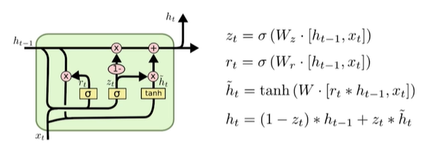
GRU (Gated Recurrent Unit)

• Simpler Architecture with two gates (Reset Gate, Update Gate)
• No cell state, just hidden state
• Generalization performance가 LSTM보다 더 좋음
  

Self-Attention

• At high level,
  • ex. The animal didn't cross the street becuase it was too tired.
  • What is it refferering to?
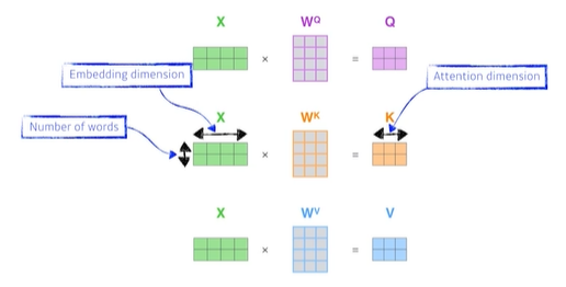
• 1 단어 당 3가지 벡터를 만들어 냄 (=3개의 뉴럴 네트워크가 있다)
  • Key vector
  • Query vector
  • Value vector
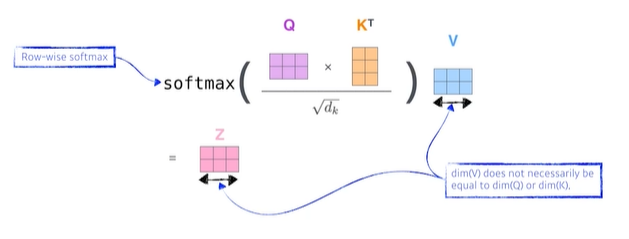
• 단어의 encoding vector를 구하는 과정
  • 1. 단어의 Score vector를 계산함. 자신의 query vector와 나머지 단어의 key vector를 내적함 -> 어떤 단어가 다른 단어들과 얼마나 align이 잘 되어있는지, 얼마나 관계가 있고, 유사도가 있고, 얼마나 관심을 가져야 할 지 볼 수 있는 지표
  • 2. Score vector를 normalize해줌. key vector의 dimension의 제곱근으로 normalize 해줌.
  • 3. 단어의 개수만큼 나온 normalized Score vector를 softmax를 취해줌
  • 4. softmax 값을 가중치로써 삼고, value vector들의 weighted sum을 구한다.
  • 행렬로 표현해보자!
    • 
    • 
• 왜 성능이 좋을까?
  • 인코딩하려는 단어와 옆에 있는 단어들에 따라서 임베딩 벡터가 달라짐 -> flexible

Multi-Headed Attention

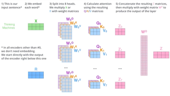
• Self Attention을 여러번 한 것
• If eight heads are used, we end up getting eight different sets of encoded vectors (attention heads)
  
• 단, 입력과 출력을 맞추어 주어야 함. linear weight matrix를 통해 dimension을 맞추어 준다.
  

Trnasformer

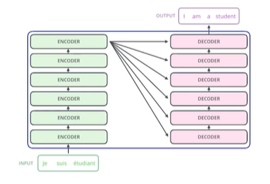
• Transformer is the first sequence transduction model based entirely on attention
• 재귀적인 구조가 없고, attention이라 불리는 모델을 사용했다.
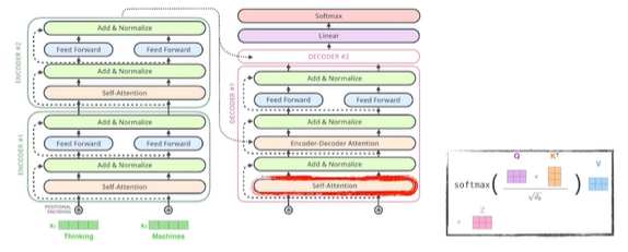
• 여러 층의 encoder (6개)와 여러 층의 decoder (6개)로 이루어져 있다. (identical but not shared)
  
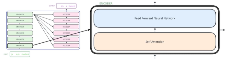
  -Encoder
  
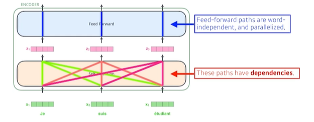
  • Self-Attention in both encoder and decoder is the conerstone of Trnasformer
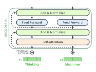
  • First, we represent each word with some embedding vectors.
    
  • Then, Trnasformer encodes each word to feature vectors with Self-Attention
    
  • Positional Encoding : Self-Attention은 order-independent, 순서에 상관없이 같은 encoding이 나옴. 그렇기 때문에 위치 정보를 담아 주어야 함.
    
• Decoder
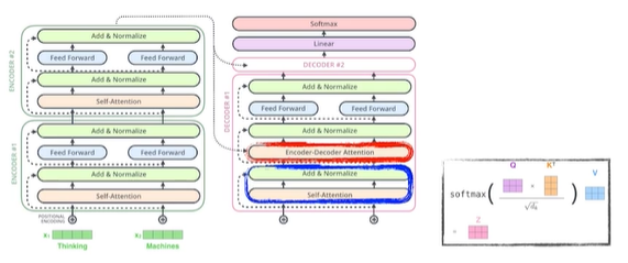
  • Encoder에서의 key와 value를 Decoder에 보냄. 왜냐하면 단어의 embedding vector를 구할 때 query, key vector를 가지고 attention을 통해서 나온 것에 value를 weighted sum해서 구했기 때문에.
  • In the Decoder, the self-attention layer is only allowed to attend to earlier positions in the output sequence which is done by masking future positions before the softmax step.
    
  • The "Encoder-Decoder Attention" layer works just like multi-headed self-attention, except it creates its Queries matrix from the layer below it, and takes Keys and Values from the encoder stack.
    
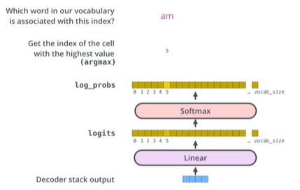
  • The final layer converts the stack of decoder outputs to the distribution over words.
    

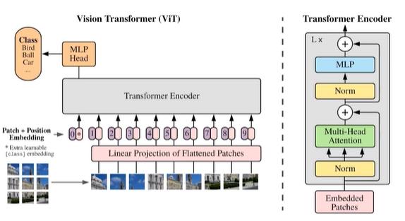
Vision Trnasformer (ViT)

• Trnasformer의 Encoder를 사용하여 이미지의 feature vector를 뽑고, 분류에 사용함.
  

DALL-E

• 주어진 문장을 바탕으로 그에 맞는 이미지를 생성함
• GPT-3 기반, GPT도 그 안에는 transformer가 있음

Day 4

강의 듣기 - Generative Model

Learning a Generative Model

• Suppose that we are given images of dogs
• We want to learn a probability distribution $p(x)$ such that
  • Generation : If we sample $\tilde{x}\sim p(x)$, $\tilde{x}$ should look like a dog
  • Density estimation : $p(x)$ should be high if x looks like a dog, and low otherwise
    • This is also known as explicit models
• Then, how can we represent $p(x)$

Autoregressive Models

• Suppose we have $28\times 28$ binary pixels.
• Our goal is to learn $P(X) = P(X_1, ..., X_{784}$ over $X\in\{0,1\}^{784}$
• How can we parametrize $P(X)$?
  • Let's use the chain rule and markov assumption to factor the joint dist'n
  • In other words,
    • $P(X_{1:784})=P(X_1)P(X_2|X_1)P(X_3|X_2)\cdots$
    • This is called an autoregressive model
    • Note that we need an ordering (ex. raster scan order) of all random variables.

AR Model - NADE

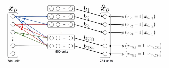
• The probability distribution of i-th pixel is
  • $p(x_i|x_{1:i-1})=\sigma(\alpha_ih_i+b_i)$ where $h_i = \sigma(W_{<i}x_{i:i-1}+c)$
• NADE is an explicit model that can compute the density of the given inputs
• BTW, how can we compute the density of the given image?
  • Suppose that we have a binary image with 784 binary pixels (i.e., $\{x_1, x_2, ..., x_{784}\}$)
  • Then, the joint probability is computed by
    • $p(x_{1:784})=p(x_1)p(x_2|x_1)p(x_3|x_1, x_2)\cdots p(x_{784}|x_{1:783})$ where each conditional probability $p(x_i|x_{1:i-1})$ is computed independently.
• In case of modeling continuous random variables, a mixture of Gaussian(MoG) can be used.
  

Summary of AR Models

• Easy to sample from
  • Sample $\tilde{x_0}\sim p(x_0)$
  • Sample $\tilde{x_1}\sim p(x_1|x_0=\tilde{x_0})$
  • $\cdots$ and so forth (in a sequential manner, hence slow)
• Easy to compute probability $p(x = \tilde{x})$
  • Compute $p(x_0 = \tilde{x_0})$
  • Compute $p(x_1 = \tilde{x_1}|x_0 = \tilde{x_0})$
  • Multiply together (sum their logarithms)
  • $\cdots$ and so forth
  • Ideally, we can compute all these terms in parallel
• Easy to be extended to continuous variables. For example, we can choose mixture of Gaussians.

Maximum Likelihood Learning

• Given a training set of examples, we can cast the generative model learning process as finding the best-approximating density model from the model family.
• Then, how can we evaluate the goodness of the approximation? (좋음의 기준을 어떻게 정할 것인가!)
  • KL-divergence
    • $P_{data}$ : data를 생성하는 분포
    • $P_{\theta}$ : $\theta$로 parameterize 되는 모델
    • $D(P_{data}\|P_{\theta}) = E_{x\sim P_{data}}\left[\log \left(\frac{P_{data}(x)}{P_{\theta}(x)}\right)\right]=E_{x\sim P_{data}}\left[\log {P_{data}(x)}\right]-E_{x\sim P_{data}}\left[\log {P_{\theta}(x)}\right]$
    • As the first term does not depend on $P_{theta}$, minimizing the KL-divergence is equivalent to maximizing the expected log-likelihood.
      $\argmin_{P_{\theta}}D(P_{data}\|P_{\theta}) \argmin_{P_{\theta}}-E_{x\sim P_{data}}\left[\log {P_{\theta}(x)}\right] = \argmax_{P_{\theta}} E_{x\sim P_{data}}\left[\log {P_{\theta}(x)}\right]$
• Approximate the expected log-likelihood $E_{x\sim P_{data}}\left[\log {P_{\theta}(x)}\right]$ with the empirical log-likelihood $E_{\mathcal{D}}\left[\log {P_{\theta}(x)}\right] = \frac{1}{|\mathcal{D}|}\sum_{x \in \mathcal{D}}\log P_{\theta}(x)$
• Maximum Likelihood Learning is then:
  $\max_{P_{\theta}}\frac{1}{|\mathcal{D}|}\sum_{x \in \mathcal{D}}\log P_{\theta}(x)$
• Problem - Variance of Monte Carlo estimate is high = data가 많지 않을 때는 정확하지 않을 수 있다:
  $V_{P}[\hat{g}] = V_P\left[\frac{1}{T}\sum_{t=1}^{T}g(x^t)\right]=\frac{V_P[g(x)]}{T}$
• For maximum likelihood learning, empirical risk minimization (ERM) is often used. 갖고 있는 데이터로만 학습을 하겠다(?)
• However, ERM often suffers from its overfitting
  • Extreme case : The model remembers all trainnig data $p(x)=\frac{1}{|\mathcal{D}|}\sum_{i=1}^{|\mathcal{D}|}\delta(x, x_i)$
  • 새로운 강아지 이미지를 만들어야 하는데 학습과정에서 본 데이터를 그대로 생성하면 의미 없다.
• To achieve better generalization, we typically restrict the hypothesis space of distributions that we search over.
• However, it could deteriorate the performance of the generative model.
• Usually, MLL is prone to under-fitting as we often use simple parametric distributions such as spherical Gaussians.
• What about other ways of measuring the similarity?
  • KL-divergence leads to maximum likelihood learning or Variational Autoencoder (VAE)
  • Jensen-Shannon divergence leads to Generative Adversarial Nework (GAN) ($D(A\|B)+D(B\|A) / 2$)
  • Wasserstein distance leads to Wasserstein Autoencoder (WAE) or Adversarial Autoencoder (AAE)

Latent Variable Models

• Is Autoencoder a generative model? No.
• What is Variational AutoEncoder (VAE)?
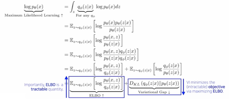
  • Variational Inference (VI)
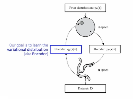
    • The goal of VI is to optimize the variational distribution that best matches the posterior distribution
      • Posterior distribution: $p_{\theta}(z|x)$
      • Variational distribution : $q_{\phi}(z|x)$
      • Posterior를 계산해야 하는데 너무 식이 복잡해서 구할 수 없을 때 상대적으로 표현력이 떨어지지만 우리가 나타낼 수 있는 Variational Dist'n을 구한다.
    • In particular, we want to find the variational distribution that minimizes the KL divergence between the true posterior.
      
      
      
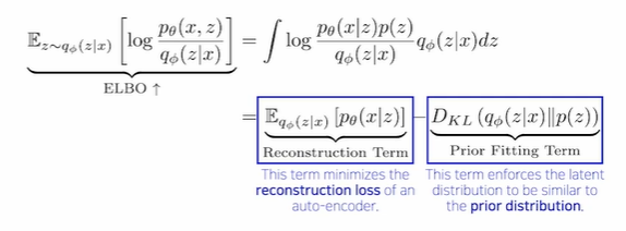
  • Key limitation
    • It is an intractable model (hard to evaluate likelihook)
    • The prior fitting term should be differentiable, hence it is hard to used diverse latent prior distributions.
    • In most cases, we use an isotropic Gaussian where we have a closed-form for the prior fitting term.
      $D_{KL}(q_{\phi}(z|x)\|\mathcal{N}(0, I)) = \frac{1}{2}\sum_{i=1}^{D}(\sigma_{z_i}^2 + \mu_{z_i}^2 - \log{\sigma_{z_i}^2}-1)$

Generative Adversarial Networks (GAN)

• $\min_G \max_D V(D, G)=\mathbb{E}_{x\sim p_{data}(x)}[\log{D(x)}] + \mathbb{E}_{z\sim p_{z}(z)}[\log{1-D(G(z))}]$
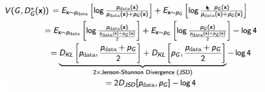
• GAN is a two player minimax game between generator and discriminator
  • Discriminator objective
    $\max_D V(D, G)=\mathbb{E}_{x\sim p_{data}}[\log{D(x)}] + \mathbb{E}_{x\sim p_{G}}[\log{1-D(x)}]$
  • The optimal discriminator is
    $D_G^*(x)=\frac{p_{data}(x)}{p_{data}(x)+p_{G}(x)}$
  • Plugging in the optimal discriminator, we get
    

Diffusion Models

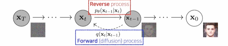
• Diffusion models progressively generate images from noise
• Forward(Diffusion) process progressively injects noise to an image.
  $p_{\theta}(x_{t-1}|x_t):=\mathcal{N}(x_{t-1};\mu_{\theta}(x_t,t),\sum_\theta (x_t,t))$
• The reverse process is learned in such a way to denoise the perturbed image back to a clean image.
  

Day 5 - Vizualization

Bar plot

• 막대의 방향에 따른 분류
  • 수직 : .bar
  • 수평 : .barh()
• Multiple bar plot
  • 쌓아서 표현하기
    • .bar()에서는 bottom 파라미터 사용
    • .barh()에서는 left 파라미터 사용
    • 위의 plot은 분포를 파악하기 힘듦
    • annotation을 달아 놓는 것이 좋음
    • Percentage Stacked Bar Chart도 좋음
  • 겹쳐서 표현하기
  • 이웃에 배치하여 표현하기