Matrix Computation

Matrix Algebra

Matrix -- The mother of all data structures. The nonmathematical uses of the word matrix reflect its Latin origins in mater, or mother.... The word has two meanings -- a representation of a linear mapping and the basis for all our existence.

Linear Systems

Linear algebra는 $Ax=b$ 형태의 the system of linear equations에 대한 성질을 탐구한다.

이 $Ax=b$는 row picture로는 n개의 plane에 대한 intersection이며, column picture로는 A의 column vectors들의 조합으로 볼 수 있다. 일반적으로는 column picture로써 문제를 주로 바라본다.

Vector Products

두 개의 Vector를 가정하자.

일반적으로 vector는 column vector를 의미한다.

• Inner product (dot product, 내적) : scalar

• Outer product (외적) : matrix

• Elementwise product (원소곱) : vector

Matrix Multiplication

$A \in \mathbb{R}^{m\times p}$, $B \in \mathbb{R}^{p\times n}$라고 하자. 이 때, $C=AB$는 다음과 같다.

모르는 사람이 없을 공식인데, 기본적으로 A의 row vector를 원소로 가지는 vector와 B의 column vector를 원소로 가지는 vector에 대해서, 원소 간 곱을 inner product라고 했을 때의 outer product로 계산된다.

또한, 다음과 같이 표현할 수도 있다.

즉, A의 column vector를 원소로 가지는 vector와 B의 row vector를 원소로 가지는 vector에 대해서, 원소 간 곱을 outer product라고 했을 때의 inner product로 계산된다.

Matrix Multiplication을 효율적이고 빠르게 하는 것이 학습 속도를 결정하기 때문에 이 부분을 열심히 파보는 것도 좋을 것 같다.

Determinant and Positive Definite

Determinant of a Matrix

A의 determinant는 A의 row vector들로 표현된 $n$-dimensional space 상의 parallelepiped $P$의 부피와 같다.

아마 Matrix를 하나의 값으로 표현한다면 가장 흔하게 사용될 값이 바로 determinant 이다. (Determinant 값이 음수라면 공간의 방향(orientation)이 뒤집힌다는 의미이다.)

Determinant와 관련된 공식은 많지만, 아래 정도만 기억해도 고차원 수학을 다룰 예정이 아니라면 별 문제는 없었던 것 같다.

• A matrix $A$ has an inverse matrix $A^{-1}$ if and only if $det(A)\ne 0$
• If $A$ is triangular, then $det(A)=a_{11}a_{22}...a_{nn}$. In Particular, $det(I_n)=1$.
• $det(AB) = det(A)det(B)$
• $tr(AB)=tr(BA)$

간혹 invese matrix를 프로그램이나 알고리즘 내에서 직접 explicit하게 계산하도록 코드를 구현하는 사람들이 있는데, 높은 확률로 뻗어버릴테니 꼭 피하길 바란다.

Symmetric Positive Definite (SPD) Matrix

Symmetric Positive Definite(SPD)는 이후 다룰 Optimization 내용에서 중요하게 사용되는 성질이다.

SPD의 정의는 다음과 같다.

• Symmetric: $A=A^T$
• Positive Definite (or positive semi-definite): if $x^TAx>0$ (or $x^TAx\ge 0$) for all nonzero $x \in \mathbb{R}^n$, denoted by $A \succ 0$ (or $A \succeq 0$).

만약 $C\in\mathbb{R}^{n\times n}$가 full rank를 가지고 $A=C^TC$이면, $A$는 SPD이다.

참고로 Covariance Matrix는 SPD이다.

where $\mathbf{x}_i = \begin{bmatrix} x_{i1} & ... & x_{ip} \end{bmatrix}^T$.

The Cholesky Factorization

The Cholesky Factorization는 SPD matrix가 갖는 중요한 성질로, 모든 SPD는 positive diagonal entry를 갖는 upper-triangular matrix로 unique하게 분해된다.

Theorem: Cholesky factorization
Every SPD matrix $A=(a_{ij})\in\mathbb{R}^{n\times n}$ has a uniqe Cholesky factorization

$A=R^TR, \qquad r_{ii} > 0$

where $R=(r_{ij})$ is an $n\times n$ upper-triangular matrix with positive diagonal entries.

위 $R$을 $A^{\frac{1}{2}}$로 표현하기도 한다.

Tests for Positive Definiteness

어떤 Matrix가 Positive Definite인지 판별하는 방법은 다음과 같 은 것들이 있다.

• All the eigenvalues of $A$ satisfy $\lambda_i>0$.

• All the upper left submatrices $A_k$ have positive determinants.

• $2\times 2$-matrix $\left[ \begin{array}{cc} a & b \\ b & c\\ \end{array} \right]$ is positive definite when $a>0$ and $ac-b^2>0$.

Linear Algebra

Linear Dependency and Basis

• The vectors $v_1, v_2, ..., v_k$에 대해 $c_1v_1 + ... + c_kv_k=0$을 만족하는 조건이 오직 $c_1=...=c_k=0$이면, 이는 linearly independent 이다. (반대는 linearly dependent)

  • 만약 $v_i$들이 linearly dependent하면, $v_i$들 중 하나($v_k$)를 나머지 vector들 $(v_1,\dots,v_{k-1},v_{k+1},\dots,v_n)$의 linear combination으로 표현할 수 있다.

• 어떤 vector space $V$에 대해, $V$ 내 모든 vector $v$를 $v_i$들의 linear combination들로 표현할 수 있는 경우, $v_i$들이 $V$를 생성(span)한다고 말한다.

• 만약 다음 조건들이 만족되는 경우 $\lbrace v_i\rbrace$를 $V$의 basis 라고 한다.

  1. $v_i$'s are linearly independent.
  2. $\lbrace v_i\rbrace$ spans the space $V$.

• Vector space $V$의 basis를 구성하는 vector의 수를 $V$의 dimension 이라고 한다.

Norms

• Let $S$ be a vector space with elements $x$.
  이 때, 다음 조건들을 만족하는 real-valued function $\Vert x \Vert$을 norm 이라고 한다:
  1. $\Vert x \Vert \ge 0$ for any $x\in S$
  2. $\Vert x \Vert=0$ if and only if $x=0$
  3. $\Vert\alpha x \Vert = \vert \alpha \vert \Vert x \Vert$, where $\alpha$ is an arbitrary scalar
  4. $\Vert x+y \Vert \le \Vert x\Vert+\Vert y\Vert$ (triangular inequality)

새로운 Norm을 만들 때, triangular inequality를 만족하는지 꼭 체크해야한다.

Vector Norms

• Vector $p$-norm: $\Vert x \Vert_p = \left( \sum_{i=1}^n \vert x_i \vert^p \right)^{1/p}$

• Manhattan: $\Vert x\Vert_1=\sum_{1\le i \le n} \vert x_i\vert$$

• Euclidian: $\Vert x \Vert_2=\sqrt{x^Tx}$

• Chebyshev: $\Vert x\Vert_\infty=\max_{1\le i \le n} \vert x_i\vert$

Matrix Norms

• Matrix $p$-norm

  $\Vert A\Vert_p = \sup_{x\ne 0}\frac{\Vert Ax\Vert_p}{\Vert x\Vert_p}$

• Frobenius norm

  $\Vert A\Vert_F=\left( \sum_{i=1}^m\sum_{j=1}^n\vert a_{ij}\vert^2 \right)^{1/2} = \sqrt{tr(A^TA)}$

Matrix Operation on Vectors

Linear Transformations

만약 특정 공간의 basis들에 대한 linear transformation ($Ax_i$) 를 안다면, 우리는 그 공간 전체에 대한 linear transformation을 알 수 있다.

• Linearity: If $x=c_1x_1+...+c_nx_n$, then $Ax = c_1(Ax_1)+...+c_n(Ax_n)$.

자주 사용되는 linear transformation으로는 Scaling, Rotation, Identity, Projection, Reflection 등이 있다.

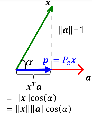
Projection Using Inner Products

WANT: project $x$ to $a$.

• $p=(x^Ta)a=(a^Tx)a=a(a^Tx)=(aaT)x=P_ax$

• $P_a=aa^T$ if $\|a\| = a^Ta = 1$

• $P_a=\frac{aa^T}{a^Ta}$ in general

  • 이 때, $P_a$를 projection matrix 라고 한다.

Least Squares

Least Squares Solution

Theorem: Least Squares Solution
The least squares solution to :

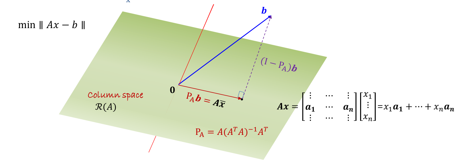
$\min \|Ax-b\| \qquad A\in \mathbb{R}^{m\times n}, \; m>n$

satisfies the following normal equation : $A^TA\bar{x} = A^Tb$

Least square 문제는 아래 figure에서 볼 수 있듯이 Ax 위로의 b의 projection 문제와 동일하다.

이는 앞으로 나올 수많은 dimension reduction 기법의 가장 기초가 된다.

• If $A^TA$ is invertible, then $\bar{x} = (A^TA)^{-1}A^Tb$

• If $p$ is the projection of b onto the column space of $A$, then $p=A\bar{x} = Pb = A(A^TA)^{-1}A^Tb$,
  where $P$ is an orthogonal projection matrix given by $A(A^TA)^{-1}A^T$

• $P\in \mathbb{R}^{n\times n}$ is said to be a projection if $P^2=P$.

• $P\in \mathbb{R}^{n\times n}$ is an orthogonal projection if $P^2=P$ and $P=P^T$.

Orthogonal Matrix

• Matrix $Q$의 column과 row vector들이 orthogonal unit vectors (orthonormal vectors)이면, i.e. $Q^TQ=QQ^T=I$, 이 때의 $Q$를 orthogonal matrix라고 한다.

Orthogonal matrix는 다음과 같은 좋은 성질을 가진다.

• $Q^T=Q^{-1}$

• $\Vert Qx\Vert = \Vert x\Vert$

• $(Qx)^T(Qy)=x^Ty$

Orthogonal matrix를 이용한 transformation은 lengths와 inner products를 보존한다.

Theorem: Orthogonal Matrix
If the columns of $Q_r=[q_1,...,q_r]\in \mathbb{R}^{n\times r}$ are an orthonormal basis for a subspace $S$, then the least squares problem $\min\|Q_rx-b\|$ becomes easy

$Q_r^TQ_r\bar{x} = Q_r^Tb \Rightarrow \bar{x}=Q_r^Tb.$

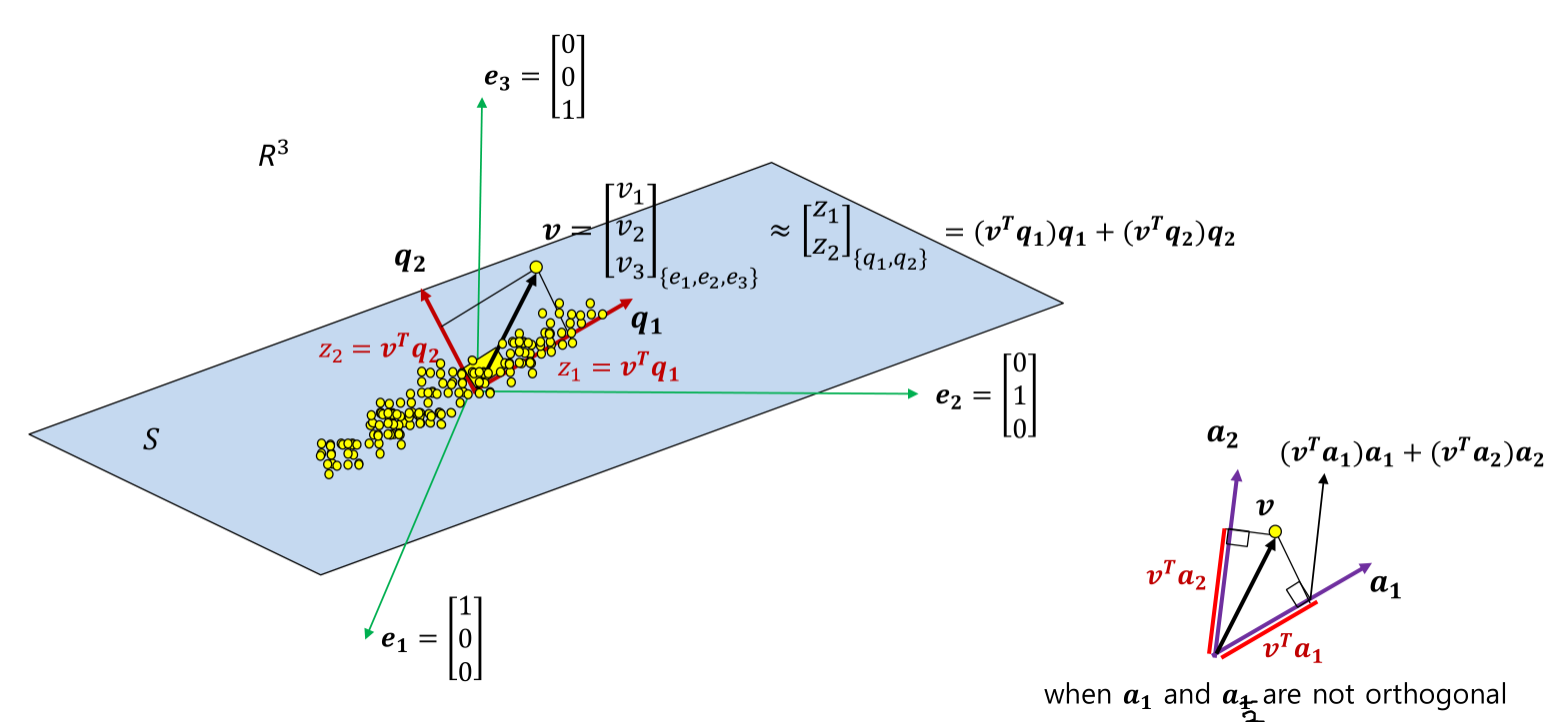
The projection of $b$ and the unique orthogonal projection matrix onto the column space $S=span\lbrace q_1,...,q_r\rbrace$ is

$p=P_sb=Q_r\bar{x}=Q_rQ_r^Tb, \quad P_s=Q_rQ_r^T=\sum_{i=1}^r q_iq_i^T$

만약 $Q=[q_1,...,q_n]\in R^{n\times n}$의 column들이 orthonormal basis이면, $b$는 다음과 같이 쓸 수 있다.

어떤 vector를 다른 basis로 표현하는 기법으로, 이 역시 dimension reduction을 포함한 feature transformation 기법의 기초가 된다.