데이터 전처리(Splitting & Scaling), 표준점수(standard score), 샘플링 편향(2)

데이터 전처리 방법을 알아본다.

• Splitting(train, test)
• Scaling

Data preprocessing

fish_length = [25.4, 26.3, 26.5, 29.0, 29.0, 29.7, 29.7, 30.0, 30.0, 30.7, 31.0, 31.0, 
                31.5, 32.0, 32.0, 32.0, 33.0, 33.0, 33.5, 33.5, 34.0, 34.0, 34.5, 35.0, 
                35.0, 35.0, 35.0, 36.0, 36.0, 37.0, 38.5, 38.5, 39.5, 41.0, 41.0, 9.8, 
                10.5, 10.6, 11.0, 11.2, 11.3, 11.8, 11.8, 12.0, 12.2, 12.4, 13.0, 14.3, 15.0]
fish_weight = [242.0, 290.0, 340.0, 363.0, 430.0, 450.0, 500.0, 390.0, 450.0, 500.0, 475.0, 500.0, 
                500.0, 340.0, 600.0, 600.0, 700.0, 700.0, 610.0, 650.0, 575.0, 685.0, 620.0, 680.0, 
                700.0, 725.0, 720.0, 714.0, 850.0, 1000.0, 920.0, 955.0, 925.0, 975.0, 950.0, 6.7, 
                7.5, 7.0, 9.7, 9.8, 8.7, 10.0, 9.9, 9.8, 12.2, 13.4, 12.2, 19.7, 19.9]

35 빙어 14 도미 데이터

import numpy as np
np.column_stack((fish_length, fish_weight)) # (smaple 개수 x feature 개수) 형태의 리스트

위와 같은 방식으로 data를 전처리할 수 있다.

Target preprocessing

타겟 데이터는 1과 0을 여러번 곱해서 만드는 것 보다 numpy의 np.ones(), np.zeros()를 사용하여 쉽게 처리할 수 있다.
두 배열을 연결할 때 class 단위로 분류하기 때문에 일차원 배열로 만들어주기 위한 함수 np.concatenate()를 사용한다.

fish_target = np.concatenate((np.ones(35), np.zeros(14)))

Data preprocessing with scikit-learn

이번엔 scikit-learn의 train_test_split()를 사용하여 데이터 전처리를 수행한다.

from sklearn.model_selection import train_test_split
trarin input, test_input, train_target, test_target = train_test_split(fish_data,
	fish_target, random_state=42) # sample을 무작위로 섞어 train, test data set 반환

train_test_split() 함수는 기본적으로 25%를 test data로 보낸다.

stratify for sampling bias

stratify는 train_test_split() 함수의 매개변수로 전체 data set에서의 class 비율에 맞게 train, test set을 나누는 역학을 한다.

train_input, test_input, train_target, test_target = train_test_split(fish_data, 
	fish_target, stratify=fish_target, random_state=42) 

인자로 target data set을 전달한다.

이전 코드에서 train test 비가 3.3:1이였지만, statify 매개변수를 조정해준 후는 2.25:1로 전체 데이터 셋과 비율이 비슷하다.

K-최근접 이웃 알고리즘(2)

이전과 같이 모델을 KNeighborsClassifier 객체로 학습한다.

from sklearn.neighbors import KNeighborsClassifier
kn = KNeighborsClassifier()
kn.fit(train_input, train_target)
kn.score(test_input, test_target) # 1.0

print(kn.predicts(([25, 150]))) # [0.]

도미 데이터를 빙어로 예측한다.

왜 이런 문제점이 나타나는 것일까?
이전 포스트에서 언급했듯이 KNeighborsClassifier 객체는 학습한 데이터 중, 가장 가까운 데이터 5개(default)를 비교하여 5개 중 더 많은 sample을 가진 class로 예측한다.
이말은 학습한 데이터의 산점도에서 예측할 도미 데이터와 가까운 5개의 데이터의 과반수 이상이 빙어 데이터 였던 것이다.

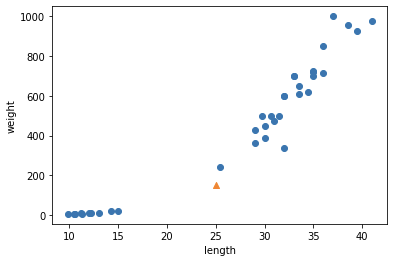
예측할 샘플의 산점도

import matplotlib.pyplot as plt
plt.scatter(train_input[:,0], train_input[:,1])
plt.scatter(25, 150, marker='^')
plt.xlabel("length")
plt.ylabel("weight")
plt.show()

최근접 5개의 sample을 표시한 산점도

object.KNeighbors() 함수는 sample을 인자로 받아 가장 가까운 sample들과의 거리, 인덱스를 리스트로 반환한다.

distances, indexes = kn.kneighbors([[25, 150]])
plt.scatter(train_input[:,0], train_input[:,1])
plt.scatter(train_input[indexes,0], train_input[indexes, 1], marker='D')
plt.xlabel("length")
plt.ylabel("weight")

이전의 산점도와 다르게 최근접 sample들을 표시하여 산점도를 표현하여 보면, 밑의 4개의 sample을 확인할 수 있다. 이는 빙어의 sample들이다.
맷플롯립으로 표현된 산점도를 보면 더 멀어보인다. 하지만 y축이 scale이 더 크기 때문에, 빙어 sample이 더 가까운 것이다.

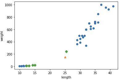
print(distances)

[[ 92.00086956 130.48375378 130.73859415 138.32150953 138.39320793]]

Scaling

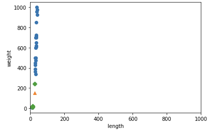
이를 명확하게 하기 위해 x축의 scale을 y축과 비슷하게 만들어주면 된다.
x축의 범위를 [0, 1,000]로 맞추어준다.
이 때 사용되는 함수는 xlim() 함수이다.

plt.scatter(train_input[:,0], train_input[:,1])
plt.scatter(25, 150. marker='^')
plt.xlim((0, 1000))
plt.scatter(train_input[indexes, 0], train_input[indexes, 1])
plt.xlabel("length")
plt.ylabel("weight")
plt.show()

이 경우 y축만 거리에 고려가 되기 때문에 이전 결과와 별반 다를게 없을 것이다. scaling을 잘못해준 것이다.

표준점수(Standard score or z 점수)

표준점수는 각 특성값이 평균에서 표준편차의 몇 배만큼 떨어져 있는지를 나타낸다.
이를 통해 실제 특성값의 크기와 상관없이 동일한 조건으로 비교할 수 있다.

mean = np.mean(train_input, axis=0) # 평균
std = np.std(train_input, axis=0) # 표준편차

axis=0 부분은 리스트의 1차원(행)을 뜻한다.

train_scaled = (train_input - mean) / std

(학습 데이터의 feature 값 - 평균) / 표준편차: 표준편차의 몇배만큼 떨어져 있는지 구한다.

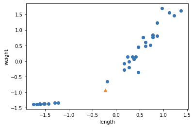
예측할 sample도 이 과정을 거쳐야 한다.

new = ([25, 150] - mean) / std
plt.scatter(train_scaled[:,0], train_scaled[:,1])
plt.scatter(new[0], new[1], makrker='^')
plt.xlabel("length")
plt.ylabel("weight")
plt.show()

Scaling 이전의 산점도랑 거의 동일하다. 하지만 y축의 범위가 달라졌다는 점이다.
그렇다면 sample을 고를 때, 눈대중으로 가까운 data를 선택할 것이다.

Scaling된 데이터로 학습 후 정확도 평가

kn.fit(train_scaled[;,0], train_scaled[:,1])
test_scaled = (test_input - mean) / std
kn.score(test_scaled, test_target) # 1.0
print(kn.predict([new])) # [1.]

predict()는 2차원 리스트를 인자로 받는다.