NLP Tutorial (8) - 임베딩 1

서론

What is embedding

임베딩은 직역하자면 끼워넣다 정도인데, 머신러닝에선 고차원의 단어나 이미지를 수학적으로 표현한 벡터 뭉치를 말한다. 이전에, 문장을 컴퓨터가 이해할 수 있는 단위인 토큰과 토큰화를 알아보았다. 하지만, 토큰화만으론 컴퓨터는 이해할 수 없다. 대신, 텍스트를 이해할 수 있는 숫자로 표현하여 던져주어야 하는데, 그것을 텍스트 벡터화(Text vectorization)라 한다.

텍스트 벡터화에는 원-핫 인코딩(One-Hot encoding), 빈도 벡터화(Count vectorization)등이 있다.

먼저, 원 핫 인코딩은 문서에 등장하는 각 단어를 고유한 인덱스로 매핑하고, 해당 인덱스의 단어가 나타나면 1을, 다른 단어는 0으로 대치하는 방법을 말한다. 예를 들어

"I like coffee", "I like bananas"

이렇게 두 문장이 있고, 인덱스는

I - 0 / like - 1 / coffee - 2 / bananas - 3

이렇게 했다고 하자. 그러면 두 문장에 대해 원-핫 인코딩을 하면 다음과 같이 표현된다.

[1, 1, 1, 0], [1, 1, 0, 1]

이렇게 변환될 것이다.

빈도 벡터화는 문서에서 단어의 빈도수를 세어 해당 단어의 빈도를 벡터로 표현하는 방식이다. 예를 들어, coffee라는 단어가 총 3번 등장하면, 해당 단어에 대한 벡터값은 3이 된다. 원-핫 인코딩과 달리, 여러 번 등장하는 단어의 빈도가 반영이 된다는 말이다.

그러나, 이러한 방법은, 벡터의 희소성(Sparsity: 0인 원소가 많은 성질)이 크다는 단점이 있다. 이게 무슨 말이냐면, 위의 예시에선 단어가 몇 개 없기에, 변환된 두 벡터가 매우 짧다. 하지만, 내가 인덱스 하려는 단어가 많아 테이블이 무진장 크다면, 벡터의 길이는 매우 길어져 연산 측면에서 비효율적이다. 게다가, 내가 유추하고자 하는 두 단어가 실제로 비슷한 의미를 갖더라도, 벡터가 텍스트의 의미를 내포하진 않기 때문에 유사도를 추정하기도 힘들다.

물론 위 두 방법은 여전히 간단하고(유사도가 아닌 단순 출현 여부나 빈도 수가 필요할 때), 데이터의 범주가 제한적인 상황에선 종종 쓰이는 방법이긴하다.

워드 임베딩(Word Embedding)

아무튼, 위에서 지적한 문제점을 극복하기 위해, Word2Vec나 fastText와 같은 단어의 의미를 학습해 표현하는 워드 임베딩 방법을 자연어 처리에선 사용한다.

워드 임베딩 기법은 단어를 고정된 길이의 실수 벡터로 표현하며, 단어의 의미를 벡터 공간에서 다른 단어와의 상대적 위치로 표현함으로써 단어 간의 관계를 출현한다.

그리고, 워드 임베딩은 고정된 임베딩을 학습하기 때문에 다의어나 문맥 정보를 다루기 어렵다는 단점이 있어 인공 신경망을 활용해 동적 임베딩(Dynamic embedding)을 사용하기도 한다.

지금부턴, 워드 임베딩 기법부터 동적 임베딩 기법까지 알아보자.

Word2Vec

Word2Vec은 2013년 구글에서 단어 간의 유사성을 측정하기 위해 분포 가설(Distributional hypothesis)을 기반으로 개발되었다.

분포 가설이란, 같은 문맥에서 자주 함께 등장하는 단어들을 서로 유사한 의미를 가질 가능성이 높다는 말이다. 예를 들어,

"내일 아이스 아메리카노를 마실 것이다."
"내일 카페 라떼를 마실 것이다."

두 문장에서 '아이스 아메리카노'와 '카페 라떼' 주변에 분포한 단어들이 동일하거나 유사하므로, 두 단어가 비슷한 의미를 가질 것이라고 예상하는 것이다.

이러한 가정을 통해 단어의 분산 표현(Distributed representation)을 학습할 수 있다. 분산 표현이란 단어를 고차원 벡터 공간에 매핑하여 단어의 의미를 담는 것을 말한다. 위 두 문장을 벡터 공간에 매핑한다면, '아이스 아메리카노'와 '카페 라떼'는 벡터 공간에서 서로 가까운 위치에 표현된다.

이러한 방법으로 빈도 기반의 벡터화 기법에서 발생한 단어의 의미 정보를 저장하지 못하는 한계를 극복 했으며, 대량의 텍스트 데이터에서도 단어 간의 관계를 파악하고 정보를 효과적으로 표현한다.

CBoW (Continuous Bag of Words)

CBoW란 주변에 있는 단어를 가지고 중간 단어를 예측하는 방법이다. 중심 단어를 맞추기 위한 주변 몇 개의 단어를 고려할지 (Window) 정해지면, 슬라이딩 윈도우(Sliding window) 기법을 통해 윈도우를 이동하며 학습한다. 아래 예시를 통해 확인해보자.

[전체 문장 : 요즘 바빠서 글을 잘 못쓰고 있어요.]

여기서 윈도우 크기가 2일 때, 학습되는 데이터들을 나열하자면

1. 요즘 바빠서 글을 - 중심 단어 : 요즘
2. 요즘 바빠서 글을 - 중심 단어 : 바빠서
3. 요즘 바빠서 글을 잘 못쓰고 - 중심 단어 : 글을
4. 바빠서 글을 잘 못쓰고 있어요. - 중심단어 : 잘
5. 글을 잘 못쓰고 있어요. - 중심단어 : 못쓰고
6. 잘 못쓰고 있어요. - 중심단어 - 있어요.

이렇게 구성된다. 그리고 다시, 이 데이터들은 다음과 같이 인공 신경망으로 투입된다.

CBoW 모델은 각 입력 단어의 원-핫 벡터를 입력값으로 받는다. 입력 문장 내 모든 단어의 임베딩 벡터의 평균을 내어 중심 단어의 임베딩 벡터를 예측한다. 입력 단어는 원-핫 벡터로 표현되어 투사층에 입력되는데, 투사층은 원-핫 벡터의 인덱스에 해당하는 임베딩 벡터를 반환하는 구조를 갖는다. 일종의 매핑층이라고 할 수 있다. 그리고 얻어진 임베딩 벡터의 평균값을 계산한 후, 평균 벡터를 가중치 행렬과 곱하여 $V$ 크기의 벡터를 얻고, 이 벡터에 소프트맥스 함수를 이용하여 중심 단어를 예측한다.

Skip-gram

Skip gram은 반대로 중심 단어를 입력 받아 주변 단어를 예측한다. CBoW와 달리, 학습 데이터 구성에 있어, 중신 단어와 주변 단어를 하나의 쌍으로 하여 학습 데이터를 구성한다. 아래 예시와 같이.

[전체 문장 : 하루에 잠은 8시간은 자야 좋은거 같아요.]

여기서 윈도우 크기가 2일 때, 학습 데이터는

1. 하루에 잠은 8시간은 - 중심 단어 : 하루에
2. 하루에 잠은 8시간은 자야 - 중심 단어 : 잠은
3. 잠은 8시간은 자야 좋은거 - 중심 단어 : 자야
4. 8시간은 자야 좋은거 같아요 - 중심 단어 : 좋은거
5. 자야 좋은거 같아요 - 중심 단어 : 같아요

이러한 차이를 보면 알 수 있듯, 하나의 중심 단어로 여러 개의 주변 단어를 예측하므로 더 많은 학습 데이터셋을 한 문장에서 추출할 수 있고 일반적으로 CBoW보다 더 좋은 성능을 보인다.

여기서,CBoW와 Skip-gram 모두 입력 단어의 원-핫 벡터를 투사층에 입력하여 해당 단어의 임베딩 벡터를 가져오고, 입력 단어의 임베딩과 가중치와의 곱셈을 통해 일정 크기의 벡터를 얻고 소프트맥스 연산을 취하는데, 말뭉치의 크기가 커질수록 사전의 크기가 커지므로 학습 속도가 느려지는 단점이 있다.

Hierachical Softmax

계층적 소프트맥스는 출력층을 이진 트리(Binary tree) 구조로 표현해 연산을 수행한다. 아래 그림과 같다.

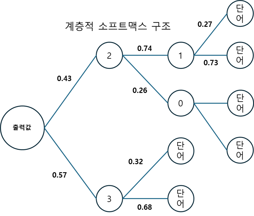
각 노드는 학습이 가능한 벡터를 가지며, 입력값은 해당 노드의 벡터와 내적값을 계산한 후 시그모이드 함수를 통해 확률을 계산한다.

잎(Leaf) 노드는 가장 깊은 노드로, 각 단어를 의미하며, 모델을 각 노드의 벡터를 최적화하여 단어를 잘 예측할 수 있게 한다. 각 단어의 확률은 경로 노드의 확률을 곱하여 구할 수 있다. 예를 들어, 최상단 단어의 확률은 $0.43 \times 0.74 \times 0.27$ 로 0.0859의 확률을 갖는다.

Code

Skip-gram

Word2Vec 모델은 학습할 단어의 수를 $V$로, 임베딩 차원을 $E$로 설정해 $W_{V \times E}$ 행렬과 $W^{'}_{E \times V}$ 행렬을 최적화하며 학습한다. 이때 $W_{V \times E}$ 행렬은 룩업(Lookuo) 연산 - 배열이나 리스트 등의 데이터 구조에서 인덱스를 이용해 해당하는 값을 찾아오는 연산 - 을 수행하는데, 임베딩 클래스로 간편하게 구현할 수 있다. 임베딩 클래스는 단어나 범주형 변수와 같은 이산 변수를 연속적인 벡터 형태로 변환해 사용할 수 있다. 연속적인 벡터 표현은 모델이 학습하는 동안 단어의 의미와 관련된 정보를 포착하고 이를 기반으로 단어 간의 유사도를 측정하고, 이산 변수 값을 연속적인 벡터로 변환하는 과정을 룩업이라 한다.

이제 임베딩 클래스 기반의 Skip-gram 클래스 코드를 살펴보자.

from torch import nn

class SimpleSkipGram(nn.Module):
    def __init__(self, vocab_size, embedding_dim):
        super(SimpleSkipGram, self).__init__()
        self.embeddings = nn.Embedding(num_embeddings=vocab_size, embedding_dim=embedding_dim)
        
        self.linear = nn.Linear(in_features=embedding_dim, out_features=vocab_size)
        
    def forward(self, input_ids):
      embeddings = self.embeddings(input_ids)
      output = self.linear(embeddings)
      return output

우선 임베딩 클래스는 단어 사전의 크기를 의미하는 임베딩 수(num_embeddings), 임베딩 차원, 입력 문장들을 일정한 길이로 맞추는 패딩 인덱스, 그리고 norm_type 등을 입력 받을 수 있다.

위 코드는 계층적 소프트맥스나 네거티브 샘플링 같은 효율적 기법이 적용되지 않은 기본 클래스로, 입력 단어와 주변 단어를 룩업 테이블에서 가져와 내적을 계산한 다음, 손실 함수를 통해 예측 오차를 최소화하는 방식으로 학습된다.

이제 사용할 데이터셋을 불러와보자. 데이터셋은 코포라 라이브러리를 이용해보자. (https://ko-nlp.github.io/Korpora/ko-docs/introduction/quicktour.html)

from torch import nn
import pandas as pd
from Korpora import Korpora
from konlpy.tag import Okt

class SimpleSkipGram(nn.Module):
    def __init__(self, vocab_size, embedding_dim):
        super(SimpleSkipGram, self).__init__()
        self.embeddings = nn.Embedding(num_embeddings=vocab_size, embedding_dim=embedding_dim)
        
        self.linear = nn.Linear(in_features=embedding_dim, out_features=vocab_size)
        
    def forward(self, input_ids):
      embeddings = self.embeddings(input_ids)
      output = self.linear(embeddings)
      return output
    
# check corpus 
corpus = Korpora.load("nsmc")
corpus = pd.DataFrame(corpus.test)

tokenizer = Okt()
tokens = [tokenizer.morphs(review) for review in corpus.text]
print(tokens[:3])

학습 데이터를 불러오고 Okt 라이브러리로 토큰화를 진행했다. 출력 결과는

    Korpora 는 다른 분들이 연구 목적으로 공유해주신 말뭉치들을
    손쉽게 다운로드, 사용할 수 있는 기능만을 제공합니다.

    말뭉치들을 공유해 주신 분들에게 감사드리며, 각 말뭉치 별 설명과 라이센스를 공유 드립니다.
    해당 말뭉치에 대해 자세히 알고 싶으신 분은 아래의 description 을 참고,
    해당 말뭉치를 연구/상용의 목적으로 이용하실 때에는 아래의 라이센스를 참고해 주시기 바랍니다.

    # Description
    Author : e9t@github
    Repository : https://github.com/e9t/nsmc
    References : www.lucypark.kr/docs/2015-pyconkr/#39

    Naver sentiment movie corpus v1.0
    This is a movie review dataset in the Korean language.
    Reviews were scraped from Naver Movies.

    The dataset construction is based on the method noted in
    [Large movie review dataset][^1] from Maas et al., 2011.

    [^1]: http://ai.stanford.edu/~amaas/data/sentiment/

    # License
    CC0 1.0 Universal (CC0 1.0) Public Domain Dedication
    Details in https://creativecommons.org/publicdomain/zero/1.0/

[nsmc] download ratings_train.txt: 14.6MB [00:01, 13.4MB/s]                                                                                                                            
[nsmc] download ratings_test.txt: 4.90MB [00:00, 13.2MB/s]                                                                                                                             
[['굳', 'ㅋ'], ['GDNTOPCLASSINTHECLUB'], ['뭐', '야', '이', '평점', '들', '은', '....', '나쁘진', '않지만', '10', '점', '짜', '리', '는', '더', '더욱', '아니잖아']]

아마 이렇게 나올 것이다.

이제 형태소를 적절히 추출했으니 단어 사전을 구축하자.

from torch import nn
import pandas as pd
from Korpora import Korpora
from konlpy.tag import Okt
from collections import Counter

class SimpleSkipGram(nn.Module):
    def __init__(self, vocab_size, embedding_dim):
        super(SimpleSkipGram, self).__init__()
        self.embeddings = nn.Embedding(num_embeddings=vocab_size, embedding_dim=embedding_dim)
        
        self.linear = nn.Linear(in_features=embedding_dim, out_features=vocab_size)
        
    def forward(self, input_ids):
      embeddings = self.embeddings(input_ids)
      output = self.linear(embeddings)
      return output

def build_vocab(corpus, n_vocab, special_tokens):
  counter = Counter()
  for tokens in corpus:
    counter.update(tokens)
  
  vocab = special_tokens
  for token, count in counter.most_common(n_vocab):
    vocab.append(token)
  return vocab
    
# check corpus 
corpus = Korpora.load("nsmc")
corpus = pd.DataFrame(corpus.test)

tokenizer = Okt()
tokens = [tokenizer.morphs(review) for review in corpus.text]


vocab = build_vocab(tokens, n_vocab=10000, special_tokens=["<pad>", "<unk>"])
token_to_id = {token: idx for idx, token in enumerate(vocab)}
id_to_token = {idx: token for idx, token in enumerate(vocab)}

print(vocab[:10])  # Print first 10 tokens in the vocabulary
print(len(vocab))  # Print the size of the vocabulary

collection의 Counter를 활용해서 build_vocab 함수로 단어 사전을 구축한다. n_vocab은 구축할 단어 사전의 크기로, 해당 크기보다 더 많은 종류의 토큰이 있다면, 가장 많이 등장한 토큰 순서로 사전을 구축한다.

special_tokens은 특별한 의미를 갖는 (사실은 특별한 존재이지만 의미가 없다는 말이 더 맞는듯 하다.) 토큰이다. 예를 들어, 여기서 <unk> 토큰은 OOV(Out of vocabulary)에 대응하기 위한 토큰으로, 단어 사전 내 없는 단어는 모두 unk로 대체되며 <pad>는 문장 길이를 맞추기 위해 채워넣는 의미 없는 토큰이다.

이제 윈도우 크기를 정하고 학습에 사용될 단어 쌍을 추출해보자.

from torch import nn
import pandas as pd
from Korpora import Korpora
from konlpy.tag import Okt
from collections import Counter

class SimpleSkipGram(nn.Module):
    def __init__(self, vocab_size, embedding_dim):
        super(SimpleSkipGram, self).__init__()
        self.embeddings = nn.Embedding(num_embeddings=vocab_size, embedding_dim=embedding_dim)
        
        self.linear = nn.Linear(in_features=embedding_dim, out_features=vocab_size)
        
    def forward(self, input_ids):
      embeddings = self.embeddings(input_ids)
      output = self.linear(embeddings)
      return output

def build_vocab(corpus, n_vocab, special_tokens):
  counter = Counter()
  for tokens in corpus:
    counter.update(tokens)
  
  vocab = special_tokens
  for token, count in counter.most_common(n_vocab):
    vocab.append(token)
  return vocab

def get_word_pairs(tokens, window_size=2):
    word_pairs = []
    for sentence in tokens:
      sentence_length = len(sentence)
      for idx, center_word in enumerate(sentence):
        window_start = max(0, idx - window_size)
        window_end = min(sentence_length, idx + window_size + 1)
        center_words = sentence[idx]
        context_words = sentence[window_start:idx] + sentence[idx+1:window_end]
        for context_word in context_words:
          word_pairs.append((center_word, context_word))
    return word_pairs
    
# check corpus 
corpus = Korpora.load("nsmc")
corpus = pd.DataFrame(corpus.test)

tokenizer = Okt()
tokens = [tokenizer.morphs(review) for review in corpus.text]


vocab = build_vocab(tokens, n_vocab=10000, special_tokens=["<pad>", "<unk>"])
token_to_id = {token: idx for idx, token in enumerate(vocab)}
id_to_token = {idx: token for idx, token in enumerate(vocab)}

word_pairs = get_word_pairs(tokens, window_size=2)
print(word_pairs[:10])  # Display first 10 word pairs

get_word_pairs 함수는 토큰을 입력받아 Skip-gram의 입력으로 사용할 수 있게 처리한다. window_size로 중심 단어에서 주변 몇개를 볼 것인지 선택한다. 출력은 다음과 같이 나올 것이다.

[('굳', 'ㅋ'), ('ㅋ', '굳'), ('뭐', '야'), ('뭐', '이'), ('야', '뭐'), ('야', '이'), ('야', '평점'), ('이', '뭐'), ('이', '야'), ('이', '평점')]

출력 단어를 보면 중심 단어와 주변 단어로 구성이 되어 있다. 임베딩 층은 단어의 인덱스만을 입력 받기 때문에, 인덱스 쌍으로 바꿔주자.

def get_index_pairs(word_pairs, token_to_id):
    index_pairs = []
    unk_index = token_to_id.get("<unk>")
    for center_word, context_word in word_pairs:
        center_index = token_to_id.get(center_word, unk_index)
        context_index = token_to_id.get(context_word, unk_index)
        index_pairs.append((center_index, context_index))
    return index_pairs

이 함수는 생성된 단어 쌍을 인덱스 쌍으로 변환하는 함수이다. 이제 학습을 위해 텐서 형식으로 다시 바꿔주자. DataLoader를 적용하면 된다.

index_pairs = get_index_pairs(word_pairs, token_to_id)
index_pairs = torch.tensor(index_pairs)
center_indices = index_pairs[:, 0]
context_indices = index_pairs[:, 1]

dataset = TensorDataset(center_indices, context_indices)
dataloader = DataLoader(dataset, batch_size=64, shuffle=True)

이제 모델 학습을 해보자.

import torch
from torch import nn
from torch import optim
import pandas as pd
from Korpora import Korpora
from konlpy.tag import Okt
from collections import Counter
from torch.utils.data import DataLoader, TensorDataset

class SimpleSkipGram(nn.Module):
    def __init__(self, vocab_size, embedding_dim):
        super(SimpleSkipGram, self).__init__()
        self.embeddings = nn.Embedding(num_embeddings=vocab_size, embedding_dim=embedding_dim)
        
        self.linear = nn.Linear(in_features=embedding_dim, out_features=vocab_size)
        
    def forward(self, input_ids):
      embeddings = self.embeddings(input_ids)
      output = self.linear(embeddings)
      return output

def build_vocab(corpus, n_vocab, special_tokens):
  counter = Counter()
  for tokens in corpus:
    counter.update(tokens)
  
  vocab = special_tokens
  for token, count in counter.most_common(n_vocab):
    vocab.append(token)
  return vocab

def get_word_pairs(tokens, window_size=2):
    word_pairs = []
    for sentence in tokens:
      sentence_length = len(sentence)
      for idx, center_word in enumerate(sentence):
        window_start = max(0, idx - window_size)
        window_end = min(sentence_length, idx + window_size + 1)
        center_words = sentence[idx]
        context_words = sentence[window_start:idx] + sentence[idx+1:window_end]
        for context_word in context_words:
          word_pairs.append((center_word, context_word))
    return word_pairs
  
def get_index_pairs(word_pairs, token_to_id):
    index_pairs = []
    unk_index = token_to_id.get("<unk>")
    for center_word, context_word in word_pairs:
        center_index = token_to_id.get(center_word, unk_index)
        context_index = token_to_id.get(context_word, unk_index)
        index_pairs.append((center_index, context_index))
    return index_pairs
  
# check corpus 
corpus = Korpora.load("nsmc")
corpus = pd.DataFrame(corpus.test)

tokenizer = Okt()
tokens = [tokenizer.morphs(review) for review in corpus.text]


vocab = build_vocab(tokens, n_vocab=10000, special_tokens=["<pad>", "<unk>"])
token_to_id = {token: idx for idx, token in enumerate(vocab)}
id_to_token = {idx: token for idx, token in enumerate(vocab)}

word_pairs = get_word_pairs(tokens, window_size=2)

index_pairs = get_index_pairs(word_pairs, token_to_id)
index_pairs = torch.tensor(index_pairs)
center_indices = index_pairs[:, 0]
context_indices = index_pairs[:, 1]

dataset = TensorDataset(center_indices, context_indices)
dataloader = DataLoader(dataset, batch_size=64, shuffle=True)

device = "cuda" if torch.cuda.is_available() else "cpu"
word2vec = SimpleSkipGram(vocab_size=len(token_to_id), embedding_dim=128).to(device)
criterion = nn.CrossEntropyLoss().to(device)
optimizer = optim.Adam(word2vec.parameters(), lr=0.1)

for epoch in range(10):
  cost = 0.0
  for input_ids, target_ids in dataloader:
    input_ids = input_ids.to(device)
    target_ids = target_ids.to(device)
    
    logits = word2vec(input_ids)
    loss = criterion(logits, target_ids)
    
    optimizer.zero_grad()
    loss.backward()
    optimizer.step()
    
    cost += loss
    
  cost = cost / len(dataloader)
  print(f"Epoch {epoch+1}, Loss: {cost.item():.4f}")

SimpleSkipGram 클래스를 활용해서 학습을 진행한다. 단어 사전 크기에 전체 단어 집합의 크기를 전달하고, 임베딩 크기는 128로 한다. 학습이 제대로 수행된 다음엔, 행렬의 임베딩 값을 추출하고 벡터 간의 코사인 유사도를 통해 단어 간의 유사도를 추출해보자. 아래는 이 실습의 전체 코드이다.

import torch
from torch import nn
from torch import optim
import numpy as np
from numpy.linalg import norm
import pandas as pd
from Korpora import Korpora
from konlpy.tag import Okt
from collections import Counter
from torch.utils.data import DataLoader, TensorDataset

class SimpleSkipGram(nn.Module):
    def __init__(self, vocab_size, embedding_dim):
        super(SimpleSkipGram, self).__init__()
        self.embeddings = nn.Embedding(num_embeddings=vocab_size, embedding_dim=embedding_dim)
        
        self.linear = nn.Linear(in_features=embedding_dim, out_features=vocab_size)
        
    def forward(self, input_ids):
      embeddings = self.embeddings(input_ids)
      output = self.linear(embeddings)
      return output

def build_vocab(corpus, n_vocab, special_tokens):
  counter = Counter()
  for tokens in corpus:
    counter.update(tokens)
  
  vocab = special_tokens
  for token, count in counter.most_common(n_vocab):
    vocab.append(token)
  return vocab

def get_word_pairs(tokens, window_size=2):
    word_pairs = []
    for sentence in tokens:
      sentence_length = len(sentence)
      for idx, center_word in enumerate(sentence):
        window_start = max(0, idx - window_size)
        window_end = min(sentence_length, idx + window_size + 1)
        center_words = sentence[idx]
        context_words = sentence[window_start:idx] + sentence[idx+1:window_end]
        for context_word in context_words:
          word_pairs.append((center_word, context_word))
    return word_pairs
  
def get_index_pairs(word_pairs, token_to_id):
    index_pairs = []
    unk_index = token_to_id.get("<unk>")
    for center_word, context_word in word_pairs:
        center_index = token_to_id.get(center_word, unk_index)
        context_index = token_to_id.get(context_word, unk_index)
        index_pairs.append((center_index, context_index))
    return index_pairs
  
def cosine_similarity(a, b):
    cosine = np.dot(b, a) / (norm(b, axis=1) * norm(a))
    return cosine
  
def top_n_index(cosine_matrix, n):
  closest_indices = cosine_matrix.argsort()[::-1]
  top_n = closest_indices[1 : n + 1]
  return top_n
  
# check corpus 
corpus = Korpora.load("nsmc")
corpus = pd.DataFrame(corpus.test)

tokenizer = Okt()
tokens = [tokenizer.morphs(review) for review in corpus.text]


vocab = build_vocab(tokens, n_vocab=10000, special_tokens=["<pad>", "<unk>"])
token_to_id = {token: idx for idx, token in enumerate(vocab)}
id_to_token = {idx: token for idx, token in enumerate(vocab)}

word_pairs = get_word_pairs(tokens, window_size=2)

index_pairs = get_index_pairs(word_pairs, token_to_id)
index_pairs = torch.tensor(index_pairs)
center_indices = index_pairs[:, 0]
context_indices = index_pairs[:, 1]

dataset = TensorDataset(center_indices, context_indices)
dataloader = DataLoader(dataset, batch_size=64, shuffle=True)

device = "cuda" if torch.cuda.is_available() else "cpu"
word2vec = SimpleSkipGram(vocab_size=len(token_to_id), embedding_dim=128).to(device)
criterion = nn.CrossEntropyLoss().to(device)
optimizer = optim.Adam(word2vec.parameters(), lr=0.1)

for epoch in range(10):
  cost = 0.0
  for input_ids, target_ids in dataloader:
    input_ids = input_ids.to(device)
    target_ids = target_ids.to(device)
    
    logits = word2vec(input_ids)
    loss = criterion(logits, target_ids)
    
    optimizer.zero_grad()
    loss.backward()
    optimizer.step()
    
    cost += loss
    
  cost = cost / len(dataloader)
  print(f"Epoch {epoch+1}, Loss: {cost.item():.4f}")
  
token_to_embedding = dict()
embedding_matrix = word2vec.embeddings.weight.data.cpu().numpy()

for word, embedding in zip(vocab, embedding_matrix):
    token_to_embedding[word] = embedding
    
index = 30
token = vocab[index]
token_embedding = token_to_embedding[token]
print(token)
print(token_embedding)

cosine_matrix = cosine_similarity(token_embedding, embedding_matrix)
top_n = top_n_index(cosine_matrix, n=10)

print(f"Top 10 similar words to {token}:")
for idx in top_n:
    similar_token = id_to_token[idx]
    similarity_score = cosine_matrix[idx]
    print(f"{similar_token}: {similarity_score:.4f}")
print("Done!")

출력은 이렇게 나올 것이다.

Top 10 similar words to 평점:
는: 0.6667
가: 0.6284
<unk>: 0.6134
때: 0.6064
...: 0.6064
.: 0.6059
정말: 0.5992
너무: 0.5948
도: 0.5940
로: 0.5794
Done!

뭔가 잘 되지 않은 느낌이다. 나중에 고찰해보도록 하겠다.