케라스 책을 보면서 어떻게 자연어를 전처리하고, AI 모델을 만드는지 공부해서 그 내용을 정리했습니다.

스팸 문자 분류

문제 정의 및 캐글에서 가져오기

주어진 텍스트를 이용해서 스팸 여부를 분석하는 문제입니다
이전 IMDB 처럼 이진 분류 문제였습니다

ham - 긍정 / spam - 부정

import pandas as pd
import numpy as np

file_path = "/content/SPAM text message 20170820 - Data.csv"
df = pd.read_csv(file_path)
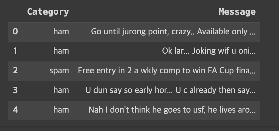
df

data를 가져오면 아래처럼 Category와 Message로 이루어진 테이블을 가져옵니다.

데이터 이해

데이터의 shape과 ham/spam 비율

데이터를 처리하기전에 데이터가 몇개 있고,
스팸문자나 다른 !,? 같은 특수 문자는 몇개 있는지 확인했습니다

df.shape # 5572, 2
df["Message"].nuinque() # 5157 -> 즉 중복 메시지가 있다
df["Category"].valie_counts() # ham-4825, spam-747 즉 spam이 적다

import plotly.express as px

fig = px.bar(df["Category"].value_counts(), width=500, height=300)
fig.show()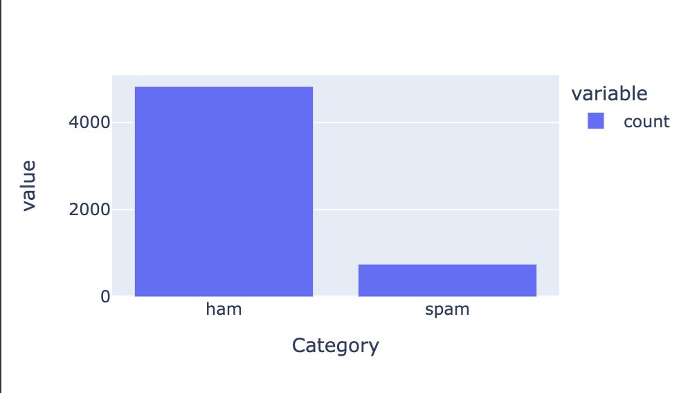

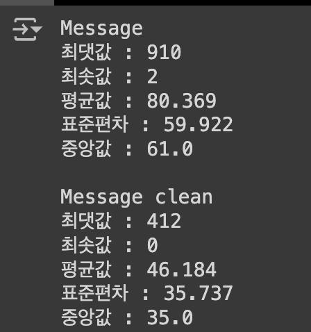
Message의 길이 및 평균 등의 describe

차고로 표준편차를 왜 구하냐고 할 수 있는데 이게 딥러닝할때 매우 중요하다!
표준편차가 크다 -> 평균에서 넓게 분포 -> 제대로 학습하는데 쉽지 않아짐;;
CV = (표준편차 / 평균) * 100

• cv < 10% => 변동성 매우 낮음
• 10 < cv < 20 => 변동성 낮음
• 20 < cv < 30 => 변동성 보통
• 30 < cv => 쓰지 마삼

import numpy as np

message_length = df["Message"].astype(str).apply(len)

printf(f'최댓값 : {np.max(message_length)}')
printf(f'최솟값 : {np.min(message_length)}')
printf(f'평균값 : {np.mean(message_length)}')
printf(f'표준편차 : {np.std(message_length)}')
printf(f'중앙값 : {np.median(message_length)}')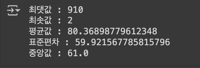

cv = (80 / 59 ) * 100 = 135.59 => cv 너무 높다!

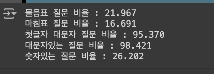
특수문자, 대문자, 소문자 비율

자연어 처리를 할때 필요없는 문자는 없애고, 대문자는 소문자로 통일해야한다
그리고 단어의 원형으로 단어를 변형해줘야한다!! => 일관성을 위해

# 물음표
qmarks = np.mean(df["Message"].apply(lambda x : '?' in x)

# 마침표
fullstop = np.mean(df["Message"].apply(lambda x : '!' in x)

# 첫번째 대문자
capital_first = np.mean(df["Message"].apply(lambda x : x[0].isupper()))

# 대문자가 몇개
capitals = np.mean(df["Message"].apply(lambda x : max([y.isupper() for y in x])))
# 숫자가 몇개
numbers = np.mean(df['Message'].apply(lambda x : max([y.isdigit() for y in x])))

가장 많이 사용된 단어 보기

wordCloud를 이용하면 많이 사용한 단어를 시각화해서 볼 수 있다

from wordcloud import WordCloud
import matplotlib.pyplot as plt

cloud = WordCloud(width=800, height=600).generate("".join(df["Message"]))

plt.figure(figsize=(20,15))
plt.imshow(cloud)
plt.axis('off')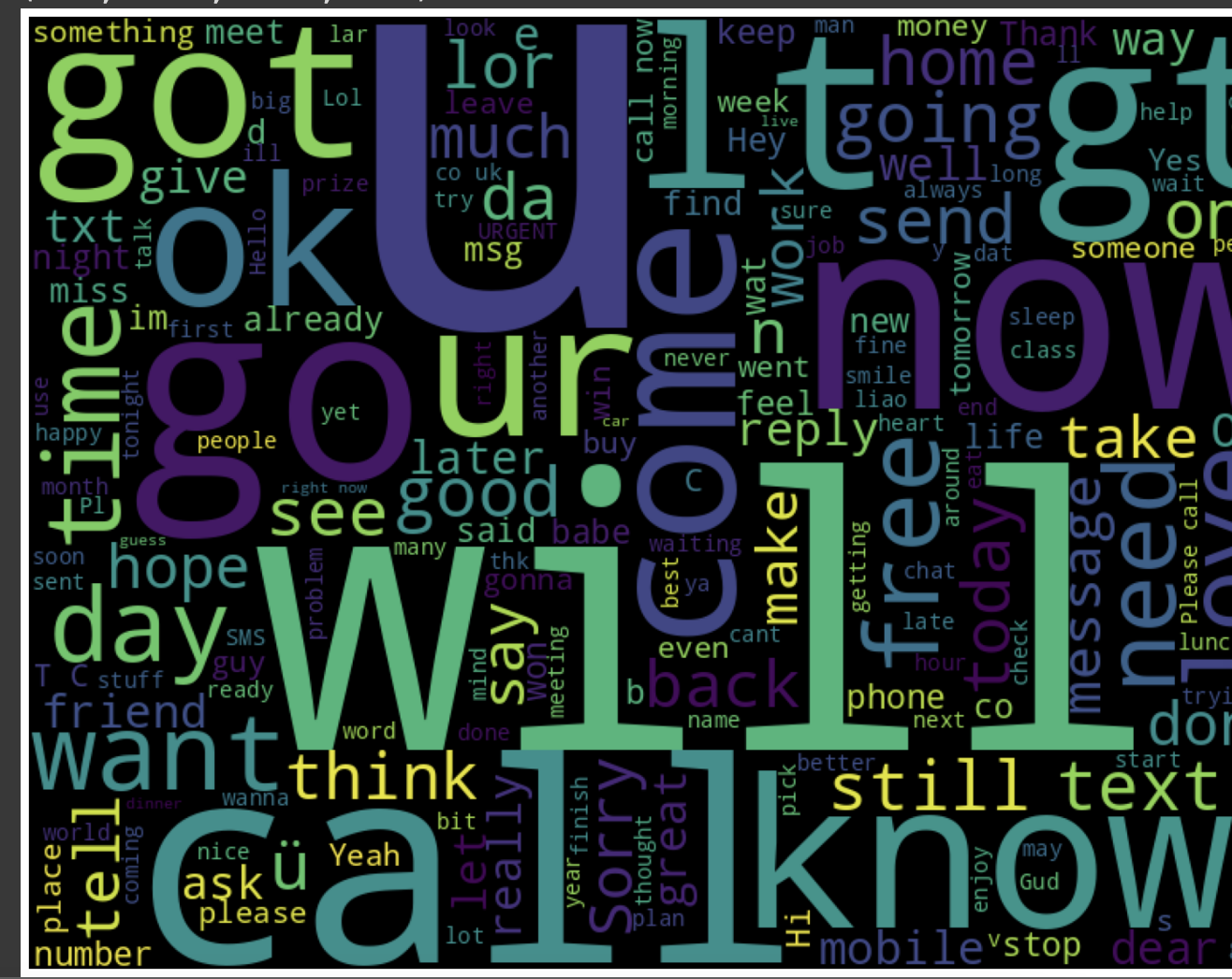

데이터 전처리

위의 내용을 보고 이제 데이터에 대해 어느정도 이해를 했습니다.
이제는 현재 나와있는 데이터를 실제로 사용할 수 있을 정도(?)의 텍스트로 변환하는 함수를 만들었습니다.

1. HTML 태그 제거 -> 이건 웹에서 크롤링 한거 아니면 제외해도 된다
2. 영문자 아닌 단어들 띄어쓰기로!
3. 소문자 변환
4. 불용어 제거
5. 단어 어간 추출 -> 단어를 기본형태로 변환해서 일관성 높이기
6. 다시 문자열로 만들어서 반환!

import re
import nltk
from nltk.corpus import stopwords

nltk.download('stopwords')
stopwords = stopwords.words('english')


def message_to_words(raw_message):
	# raw_message = BeautifulSoup(row_message, 'html_parser').get_text()
    letters_only = re.sub('[^a-zA-Z]', ' ', raw_message)

	words = letters_only.lower().split()
    
    meaningful_words = [w for w in words if w not in stopwords]
    
    steming_words = [stemmer.stem(w) for w in meaningful_words]
    return (' '.join(steming_words))

데이터 병렬 처리

현재는 데이터가 5500개 정도만 되서 괜찮지만 실제 리뷰 데이터는 10만개 이상일 수도 있다
이때 함수의 처리 속도를 높이는 방법 중 하나인 병렬 처리를 사용했다!

from multiprocessing import Pool

def _apply_df(args):
	df, func, kwargs = args
    return df.apply(func, **kwargs)
    
def apply_by_multiprocessing(df, func, **kwargs):
	workers = kwargs.pop("workers")
    pool = Pool(processes=workers)
    result = pool.map(_apply_df, [d, func, kwargs for d in np.array_split(df, workers)])
    pool.close()
    return pd.concat(list(result)
    
clean_train_message = apply_by_multiprocessing(df['Message'], message_to_words, workers=4)
df['Message_clean'] = clean_train_message

Message_clean 부분을 보면 데이터가 원형과 달라진 부분을 볼 수 있습니다

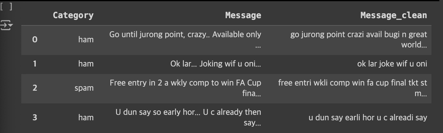
그 이후 다시 메시지를 각 분석해보면 이렇게 나온다!

라벨 데이터 인코딩

일단 라벨 데이터를 1,0으로 변형했습니다.
이때 우리가 찾고자 하는 spam이 기준이라 spam을 1로 만들었습니다.

df["Category"].apply(lambda x : 1 if x == 'spam" else 0)

중복된 데이터 제거

df.drop_duplicates(subset=["Message_clean"], inplace=True)

빈 데이터 제거

df.sort_values(by='Message_claen', ascending=True)
df = df.drop(253)

훈련 / 테스트 데이터 분리

from sklearn.model_selection import train_test_split

x_data = df["Message_clean"]
y_data = df["Category"]

x_train, x_test, y_train, y_test = train_test_split(x_data, y_data, test_size=0.2, random_state=42)

이러면 훈련 4044개와 테스트 1011개로 데이터가 나눠집니다

토큰화

단어를 이제 각 고유한 인덱스와 매칭해주는 작업을 해야한다

입력에는 당연하지만 정수나 실수만 가능해서;;

from tensorflow.keras.preprocessing.text import Tokenizer

tokeinizer = Tokenizer()
tokenizer.fit_on_texts(x_train)

x_train_tokenizer = tokenizer.texts_to_sequences(x_train)

index_to_word = tokenizer.index_word
print(index_to_word)

패딩처리

이제 숫자로 변형을 했으면 각 입력데이터의 길이를 맞춰줘야한다!
이때 패딩처리를 하는데 기본이 pre라 앞에 채워집니다

이때 최대 길이를 지정해야하는데 현재는 412가 최대길이, 평균이 46이라
대략 200으로 길이를 맞췄습니다

from tensorflow.keras.preprocessing.sequence import pad_sequences

max_len = 200
x_train_padded = pad_sequences(x_train_tokenizer, maxlen=max_len)

AI 모델링

from tensorflow.keras.callbacks import EarlyStopping, ModelCheckpoint

early_stopping = EarlyStopping(monitor='val_loss', patience=5)
modelcheckpoint = ModelCheckpoint(filepath='best_checkpoint_model.h5',
                                  monitor='val_loss',
                                  save_weights_only=True, # 가중치만
                                  save_best_only=True, # 최고의 모델만
                                  verbose=1) # 결과 보여주기

from tensorflow.keras.models import Sequential
from tensorflow.keras.layers import LSTM, Embedding, Dense

vocab_size = len(index_to_word) + 1 # 단어장
embedding_dim = 32
hidden_units=32

model = Sequential()
model.add(Embedding(vocab_size, embedding_dim))
model.add(LSTM(hidden_units))
model.add(Dense(1, activation='sigmoid'))

model.compile(optimizer='adam', loss='binary_crossentropy', metrics=['acc'])

history = model.fit(x_train_padded, y_train, validation_split=0.2, epochs=50, batch_size=32, callbacks=[early_stopping, modelcheckpoint])

acc: 0.9994 - val_loss: 0.0933 - val_acc: 0.9802

꽤나 정확한 결과가 나와서 만족했다^^
사실 test데이터를 전처리 안해서 따로 evaluate를 안했지만
다음는 전처리 다 하고 데이터 나눠야할거 같네요...