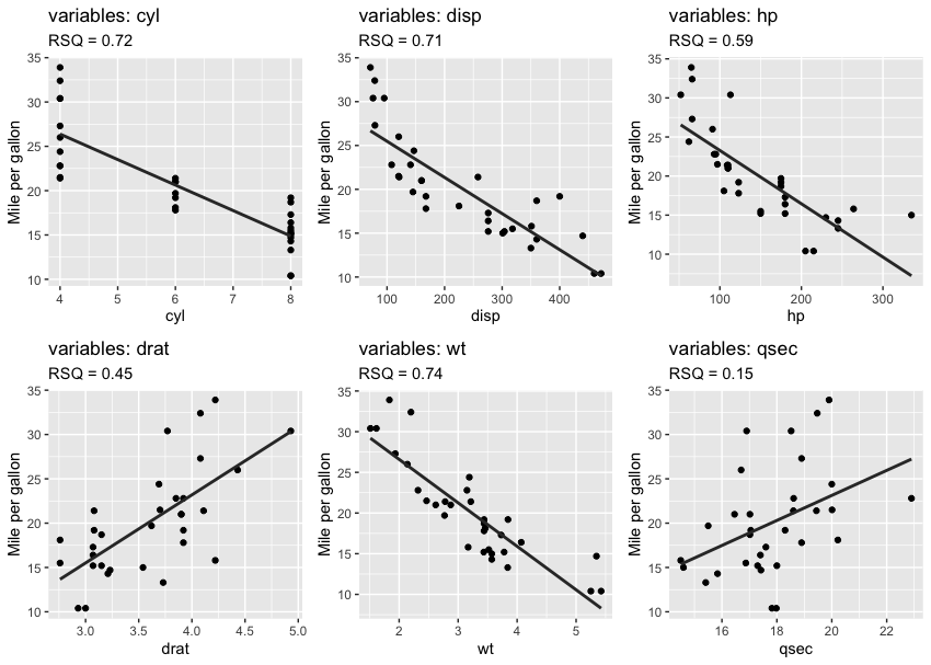
변수를 벡터로 받아서 플롯을 자동으로 작성하게 함
updated: 1st April 2023
- set_names를 사용하지 않고 데이터 슬라이싱으로 처리함
- 하나의 함수로 처리함
library(tidyverse)
# prep. data
mdf <- mtcars
# conditions
# ind: cyl, disp, hp, drat, wt, qsec
# resp: mpg

# extract colnames
inds <- colnames(mdf)[2:7]

# build function
autoPlotFun <- function(x){

  # slicing data with variable selected
  oo <- mdf[, c('mpg',x)]
  colnames(oo) <- c("mpg", "vars")

  # linear regression model and r-squared value extraction
  mod <- lm(mpg ~ vars, data = oo)
  rsqValue = summary(mod)[["adj.r.squared"]]

  # draw scattered plot with annotation of r squared value on subtitle position
  ggplot(oo, aes(vars, mpg)) +
    geom_point() +
    geom_smooth(method = 'lm', formula = 'y~x', se = FALSE, color ="grey20") +
    labs(x = paste0(x),
         y = 'Mile per gallon',
         title = paste0("variables: ", x),
         subtitle = paste0("RSQ = ", round(rsqValue, digits = 2)))

}

lapply(inds, autoPlotFun) -> plotList
cowplot::plot_grid(plotlist = plotList, ncol = 3)
- old version
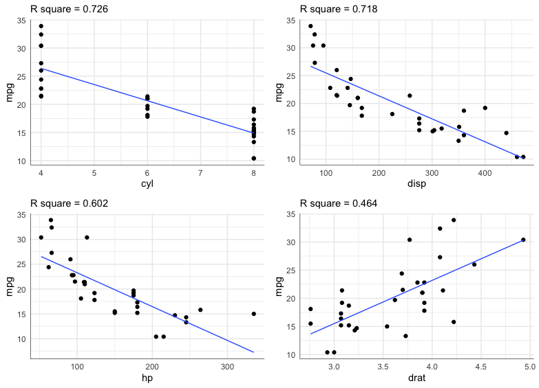
library(tidyverse)
mtcars
# dependent variables (response) : mpg
# independent variables (explanatory variables): cyl, disp, hp, drat, wt
mtcars[, c(1, 2, 3, 4, 5)] -> df
# call dependent (resp) and independent (expl) variables
resp = set_names(names(df)[1])
expl = set_names(names(df)[2:ncol(df)])
# Calculation of r square values
fun1 <- function(x, y) {
  data.frame(y = df[y][[1]],
             x = df[x][[1]]) %>%
    lm(x ~ y, data = .) %>%summary() -> a
  a$r.squared -> b
  return(b)
}
# function to draw scatter plot with regression
fun2 <- function(x, y) {
  fun1(x, y) -> r2
  ggplot(df, aes(.data[[x]], .data[[y]])) +
    geom_point() +
    geom_smooth(method = 'lm', se = F, lwd = .5, formula = y ~ x) +
    labs(subtitle = paste0("R square = ", round(r2, digits = 3))) +
    theme_minimal() +
    theme(axis.line = element_line(size = .2))
}
# create each plots and put all plot in a object
allplot = map(expl, ~fun2(.x, resp[1]))
# call out all plot using plot_grid
cowplot::plot_grid(plotlist = allplot)
data scientist