DDPM 코드 구현

유승한·2024년 10월 21일

딥러닝

목록 보기

15/15

해당 포스트는 The Annotated Diffusion Model 를 참고하여 작성되었습니다.
본 포스트의 코드는 해당 깃허브 링크에서 확인하실 수 있습니다.
DDPM의 기본 개념은 Diffusion Model 포스트를 통해 확인하실 수 있습니다.

인공신경망

인공신경망은 특정 time step에 노이즈가 포함된 이미지를 받아 예측된 noise를 반환해야합니다. 여기서 예측된 노이즈는 입력 이미지와 같은 크기로 출력됩니다. 신경망의 입력과 출력이 같아야하므로 Autoencoder가 떠오를 수 있습니다. Autoencoder의 특징으로 bottleneck이 있습니다. Autoencoder에서 인코더는 입력 이미지를 잡음 벡터로 축소하고 디코더를 통해 해당 잡음 벡터를 같은 크기의 이미지로 복원합니다. 이때 신경망은 bottleneck 레이어로 하여금 중요한 정보를 유지해야합니다.

따라서 이러한 요구사항으로 인해 아키텍쳐로 U-NET이 사용됩니다. U-NET은 일반적인 Autoencoder처럼 가운데 bottleneck 지점이 있어, 네트워크가 중요한 정보만 학습할 수 있도록 합니다. 특히, U-NET은 인코더와 디코더 사이에 residual connecions(잔차)를 도입해 학습 과정을 개선시켰습니다.

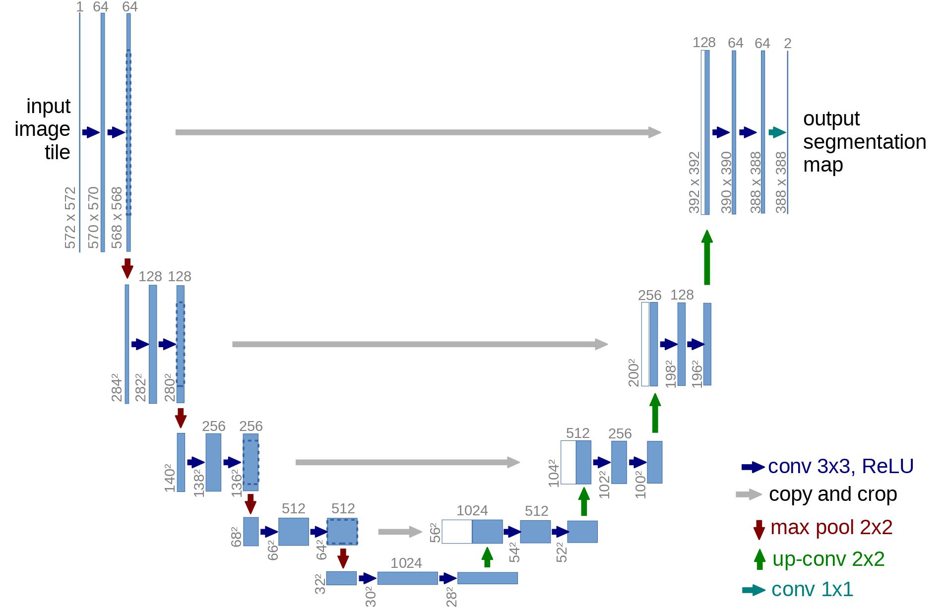
U-NET은 입력이미지를 다운샘플한 뒤에 업샘플을 합니다.

Network helpers

U-NET을 구현하기 위해 Network helper을 먼저 구현하였습니다. 특히 Residual 모듈을 정의함으로써 특정 함수의 출력의 입력으로 사용할 수 있게끔 하였습니다.

def exists(x):
    return x is not None

def default(val, d):
    if exists(val):
        return val
    return d() if isfunction(d) else d

def num_to_groups(num, divisor):
    groups = num // divisor
    remainder = num % divisor
    arr = [divisor] * groups
    if remainder > 0:
        arr.append(remainder)
    return arr

class Residual(nn.Module):
    def __init__(self, fn):
        super().__init__()
        self.fn = fn

    def forward(self, x, *args, **kwargs):
        return self.fn(x, *args, **kwargs) + x

def Upsample(dim, dim_out=None):
    return nn.Sequential(
        nn.Upsample(scale_factor=2, mode="nearest"),
        nn.Conv2d(dim, default(dim_out, dim), 3, padding=1),
    )

def Downsample(dim, dim_out=None):
    # No More Strided Convolutions or Pooling
    return nn.Sequential(
        Rearrange("b c (h p1) (w p2) -> b (c p1 p2) h w", p1=2, p2=2),
        nn.Conv2d(dim * 4, default(dim_out, dim), 1),
    )

Position embeddings

인공신경망의 파라미터(노이즈 정도)는 시간을 넘어 공유되기 때문에, DDPM의 저자는 Transformer에서 영감을 받아 t를 인코딩하기 위해 sinusoidal position embeddings를 이용하였습니다. sinusoidal position embeddings은 (batch_size, 1) 형태의 텐서를 입력으로 받고, (batch_size, dim)으로 변환합니다. 이때 dim은 position embeddings의 차원이라 볼 수 있습니다. 이는 각 residual block시간 정보를 반영하는데 사용됩니다.

class SinusoidalPositionEmbeddings(nn.Module):
    def __init__(self, dim):
        super().__init__()
        self.dim = dim

    def forward(self, time):
        device = time.device
        half_dim = self.dim // 2
        embeddings = math.log(10000) / (half_dim - 1)
        embeddings = torch.exp(torch.arange(half_dim, device=device) * -embeddings)
        embeddings = time[:, None] * embeddings[None, :]
        embeddings = torch.cat((embeddings.sin(), embeddings.cos()), dim=-1)
        return embeddings

ResNet block

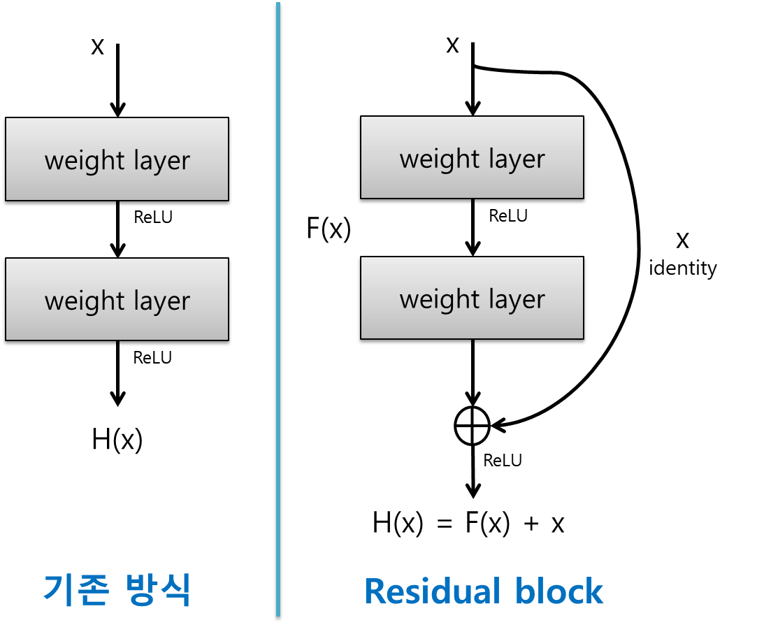
왼쪽은 Plane layer, 오른쪽은 Residual Block으로 두 구조의 차이점은 동일한 연산을 하고 Residual Block과 같은 경우에 Input인 x를 더한다는 점입니다. 단순히 Input을 더하는 것만으로 Skip Connecition을 통해 각각의 layer/block 들이 작은 정보만을 추가적으로 학습하도록 합니다. 즉 기존에 학습된 x를 추가함으로써 x만큼을 제외한 나머지 F(x)만을 학습하면 되므로 학습량이 상대적으로 줄어드는 효과가 있습니다.

DDPM의 저자는 Wide ResNet block 블록을 이용했지만 Phil Wang은 standard convolutional layer을

weight standardized 버전으로 변경하였습니다. 이는 group normalization과 함께했을 때 더 뛰어난 성과를 보인다고 합니다.

class WeightStandardizedConv2d(nn.Conv2d):
    """
    https://arxiv.org/abs/1903.10520
    weight standardization purportedly works synergistically with group normalization
    """

    def forward(self, x):
        eps = 1e-5 if x.dtype == torch.float32 else 1e-3
				
				# 가중치 텐서 self.weight의 평균과 분산을 계산하고, 이를 이용해 가중치를 표준화합니다.
        weight = self.weight
        # reduce: 가중치의 평균과 분산을 특정 차원(o)을 기준으로 구합니다. 여기서 o는 출력 채널에 해당합니다.
        mean = reduce(weight, "o ... -> o 1 1 1", "mean")
        var = reduce(weight, "o ... -> o 1 1 1", partial(torch.var, unbiased=False))
        normalized_weight = (weight - mean) / (var + eps).rsqrt()
				
				# 표준화된 가중치와 입력을 사용해 F.conv2d를 통해 합성곱 연산을 수행합니다.
        return F.conv2d(
            x,
            normalized_weight,
            self.bias,
            self.stride,
            self.padding,
            self.dilation,
            self.groups,
        )

class Block(nn.Module):
    def __init__(self, dim, dim_out, groups=8):
        super().__init__()
        # WeightStandardizedConv2d를 사용한 2D 합성곱 층입니다.
        self.proj = WeightStandardizedConv2d(dim, dim_out, 3, padding=1) 
        # GroupNorm을 사용해 출력 채널을 그룹으로 묶어 정규화합니다.
        self.norm = nn.GroupNorm(groups, dim_out)
        # SiLU 활성화 함수(Sigmoid Linear Unit)를 사용합니다.
        self.act = nn.SiLU()
		
		# 입력을 합성곱과 정규화를 거쳐 활성화 함수를 통과시킵니다.
    def forward(self, x, scale_shift=None):
        x = self.proj(x)
        x = self.norm(x)

        if exists(scale_shift):
            scale, shift = scale_shift
            x = x * (scale + 1) + shift

        x = self.act(x)
        return x

class ResnetBlock(nn.Module):
    """https://arxiv.org/abs/1512.03385"""

    def __init__(self, dim, dim_out, *, time_emb_dim=None, groups=8):
        super().__init__()
        self.mlp = (
            nn.Sequential(nn.SiLU(), nn.Linear(time_emb_dim, dim_out * 2))
            if exists(time_emb_dim)
            else None
        )

        self.block1 = Block(dim, dim_out, groups=groups)
        self.block2 = Block(dim_out, dim_out, groups=groups)
        # 입력과 출력의 차원이 다를 경우, self.res_conv를 사용해 입력을 dim_out에 맞게 변환합니다. 
        # 차원이 동일하면 단순히 Identity를 사용해 입력을 그대로 전달합니다.
        self.res_conv = nn.Conv2d(dim, dim_out, 1) if dim != dim_out else nn.Identity()

    def forward(self, x, time_emb=None):
        scale_shift = None
        if exists(self.mlp) and exists(time_emb):
            time_emb = self.mlp(time_emb)
            time_emb = rearrange(time_emb, "b c -> b c 1 1")
            scale_shift = time_emb.chunk(2, dim=1)

        h = self.block1(x, scale_shift=scale_shift)
        h = self.block2(h)
        return h + self.res_conv(x)

Attention Module

DDPM 저자는 convolutional block 사이에 Attention 모듈을 추가하였습니다. Attention은 Transformer에서 따왔으며 Phil Wang은 attention의 2가지 변형을 채용했습니다. 하나는 regular multi-head self-attention이며 두번째는 linear attention variant입니다. Attention 메커니즘은 **wonderful blog post** 해당 블로그 포스트에서 볼 수 있습니다.

class Attention(nn.Module):
    def __init__(self, dim, heads=4, dim_head=32):
        super().__init__()
        self.scale = dim_head**-0.5
        self.heads = heads
        hidden_dim = dim_head * heads
        self.to_qkv = nn.Conv2d(dim, hidden_dim * 3, 1, bias=False)
        self.to_out = nn.Conv2d(hidden_dim, dim, 1)

    def forward(self, x):
        b, c, h, w = x.shape
        qkv = self.to_qkv(x).chunk(3, dim=1)
        q, k, v = map(
            lambda t: rearrange(t, "b (h c) x y -> b h c (x y)", h=self.heads), qkv
        )
        q = q * self.scale

        sim = einsum("b h d i, b h d j -> b h i j", q, k)
        sim = sim - sim.amax(dim=-1, keepdim=True).detach()
        attn = sim.softmax(dim=-1)

        out = einsum("b h i j, b h d j -> b h i d", attn, v)
        out = rearrange(out, "b h (x y) d -> b (h d) x y", x=h, y=w)
        return self.to_out(out)

class LinearAttention(nn.Module):
    def __init__(self, dim, heads=4, dim_head=32):
        super().__init__()
        self.scale = dim_head**-0.5
        self.heads = heads
        hidden_dim = dim_head * heads
        self.to_qkv = nn.Conv2d(dim, hidden_dim * 3, 1, bias=False)

        self.to_out = nn.Sequential(nn.Conv2d(hidden_dim, dim, 1), 
                                    nn.GroupNorm(1, dim))

    def forward(self, x):
        b, c, h, w = x.shape
        qkv = self.to_qkv(x).chunk(3, dim=1)
        q, k, v = map(
            lambda t: rearrange(t, "b (h c) x y -> b h c (x y)", h=self.heads), qkv
        )

        q = q.softmax(dim=-2)
        k = k.softmax(dim=-1)

        q = q * self.scale
        context = torch.einsum("b h d n, b h e n -> b h d e", k, v)

        out = torch.einsum("b h d e, b h d n -> b h e n", context, q)
        out = rearrange(out, "b h c (x y) -> b (h c) x y", h=self.heads, x=h, y=w)
        return self.to_out(out)

Group normalization

DDPM 저자는 convolutional/ attention 레이어에 Group Normalization을 사용하였습니다. 해당 코드에서는 PreNorm 클래스를 정의함으로써 Attention 레이어 전에 groupnorm을 수행합니다.

Group Normalization은 채널 방향으로 group을 지어서 normalizaiton을 진행하며, 소규모 배치크기에서 안정적이고 효율적입니다. 다른 종류의 normalizaiton은 해당 포스트에서 확인할 수 있습니다.

class PreNorm(nn.Module):
    def __init__(self, dim, fn):
        super().__init__()
        self.fn = fn
        self.norm = nn.GroupNorm(1, dim)

    def forward(self, x):
        x = self.norm(x)
        return self.fn(x)

Conditional U-Net

이것으로 모든 블록들을 정의했으며 이제 인공신경망을 정의할 차례입니다. 네트워크의 역할은 $*ϵ_θ(x_t,t)*$ 으로, 노이즈가 섞인 이미지의 배치와 그에 해당하는 노이즈 수준을 입력 받아 입력에 추가된 노이즈를 출력하는 것입니다.

입력

노이즈가 섞인 이미지 배치 : 형태는 (batch_size, num_channels, height, width)
노이즈 수준 배치 : 형태는 (batch_size, 1)로, 각 이미지에 대한 노이즈 수준을 나타냅니다. 배치 크기 만큼의 노이즈 수준이 있으며, 각 노이즈 값은 해당 이미지에 적용된 노이즈 강도를 나타냅니다.

네트워크

convolutional layer
다운샘플링 단계
- 2개의 ResNet blocks + groupnorm + attention + residual connection + downsample operation
중간 단계
- ResNet blocks + attention
업샘플링 단계
- 2개의 ResNet blocks + groupnorm + attention + residual connection + upsample operation
  
  residual connection은 정보 손실 없이 네트워크를 복원하기 위한 용도이고 attention은 중요한 위치 정보에 집중해 복원과정에서 이미지의 복잡한 패턴을 학습하는데 사용됩니다.
출력 단계
- ResNet blocks + convolution layer
- ResNet block을 통해 네트워크의 출력을 최종적으로 조정하고 convolution 연산을 통해 출력을 생성합니다. 생성된 출력은 입력 이미지와 동일한 크기를 가지며 네트워크가 예측한 노이즈가 더해진 이미지를 나타냅니다.

class Unet(nn.Module):
    def __init__(
        self,
        dim,
        init_dim=None,
        out_dim=None,
        dim_mults=(1, 2, 4, 8),
        channels=3,
        self_condition=False,
        resnet_block_groups=4,
    ):
        super().__init__()

        # determine dimensions
        self.channels = channels
        self.self_condition = self_condition
        input_channels = channels * (2 if self_condition else 1)

        init_dim = default(init_dim, dim)
        self.init_conv = nn.Conv2d(input_channels, init_dim, 1, padding=0) # changed to 1 and 0 from 7,3

        dims = [init_dim, *map(lambda m: dim * m, dim_mults)]
        in_out = list(zip(dims[:-1], dims[1:]))

        block_klass = partial(ResnetBlock, groups=resnet_block_groups)

        # time embeddings
        time_dim = dim * 4

        self.time_mlp = nn.Sequential(
            SinusoidalPositionEmbeddings(dim),
            nn.Linear(dim, time_dim), # 시간임베딩의 차원을 확장
            nn.GELU(), # 활성화 함수
            nn.Linear(time_dim, time_dim), # 고차원 벡터를 선형 변환, 추가적인 학습을 통해 시간 정보를 더욱 구체적으로 변환
        )

        # layers
        self.downs = nn.ModuleList([])
        self.ups = nn.ModuleList([])
        num_resolutions = len(in_out)

        for ind, (dim_in, dim_out) in enumerate(in_out):
            is_last = ind >= (num_resolutions - 1)

            self.downs.append(
                nn.ModuleList(
                    [
                        block_klass(dim_in, dim_in, time_emb_dim=time_dim),
                        block_klass(dim_in, dim_in, time_emb_dim=time_dim),
                        Residual(PreNorm(dim_in, LinearAttention(dim_in))),
                        Downsample(dim_in, dim_out)
                        if not is_last
                        else nn.Conv2d(dim_in, dim_out, 3, padding=1),
                    ]
                )
            )

        mid_dim = dims[-1]
        self.mid_block1 = block_klass(mid_dim, mid_dim, time_emb_dim=time_dim)
        self.mid_attn = Residual(PreNorm(mid_dim, Attention(mid_dim)))
        self.mid_block2 = block_klass(mid_dim, mid_dim, time_emb_dim=time_dim)

        for ind, (dim_in, dim_out) in enumerate(reversed(in_out)):
            is_last = ind == (len(in_out) - 1)

            self.ups.append(
                nn.ModuleList(
                    [
                        block_klass(dim_out + dim_in, dim_out, time_emb_dim=time_dim),
                        block_klass(dim_out + dim_in, dim_out, time_emb_dim=time_dim),
                        Residual(PreNorm(dim_out, LinearAttention(dim_out))),
                        Upsample(dim_out, dim_in)
                        if not is_last
                        else nn.Conv2d(dim_out, dim_in, 3, padding=1),
                    ]
                )
            )

        self.out_dim = default(out_dim, channels)

        self.final_res_block = block_klass(dim * 2, dim, time_emb_dim=time_dim)
        self.final_conv = nn.Conv2d(dim, self.out_dim, 1)

    def forward(self, x, time, x_self_cond=None):
        if self.self_condition:
            x_self_cond = default(x_self_cond, lambda: torch.zeros_like(x))
            x = torch.cat((x_self_cond, x), dim=1)

        x = self.init_conv(x)
        r = x.clone()

        t = self.time_mlp(time)

        h = []

        for block1, block2, attn, downsample in self.downs:
            x = block1(x, t)
            h.append(x)

            x = block2(x, t)
            x = attn(x)
            h.append(x)

            x = downsample(x)

        x = self.mid_block1(x, t)
        x = self.mid_attn(x)
        x = self.mid_block2(x, t)

        for block1, block2, attn, upsample in self.ups:
            x = torch.cat((x, h.pop()), dim=1)
            x = block1(x, t)

            x = torch.cat((x, h.pop()), dim=1)
            x = block2(x, t)
            x = attn(x)

            x = upsample(x)

        x = torch.cat((x, r), dim=1)

        x = self.final_res_block(x, t)
        return self.final_conv(x)

Foward Diffusion Process

Foward Process는 실제 이미지에서 time step에 따른 variance schedule을 통해 점진적으로 노이즈를 추가합니다. DDPM 저자는 linear schedule 기법을 이용했습니다.

We set the forward process variances to constants increasing linearly from
$β_1=10^{−4}~to~β_T=0.02$

하지만 후에는 cosaine schedule을 사용하는 것이 우수하다고 밝혀졌습니다.

def cosine_beta_schedule(timesteps, s=0.008):
    """
    cosine schedule as proposed in https://arxiv.org/abs/2102.09672
    """
    steps = timesteps + 1
    x = torch.linspace(0, timesteps, steps)
    alphas_cumprod = torch.cos(((x / timesteps) + s) / (1 + s) * torch.pi * 0.5) ** 2
    alphas_cumprod = alphas_cumprod / alphas_cumprod[0]
    betas = 1 - (alphas_cumprod[1:] / alphas_cumprod[:-1])
    
    return torch.clip(betas, 0.0001, 0.9999)

def linear_beta_schedule(timesteps):
    beta_start = 0.0001
    beta_end = 0.02
    return torch.linspace(beta_start, beta_end, timesteps)

def quadratic_beta_schedule(timesteps):
    beta_start = 0.0001
    beta_end = 0.02
    return torch.linspace(beta_start**0.5, beta_end**0.5, timesteps) ** 2

def sigmoid_beta_schedule(timesteps):
    beta_start = 0.0001
    beta_end = 0.02
    betas = torch.linspace(-6, 6, timesteps)
    return torch.sigmoid(betas) * (beta_end - beta_start) + beta_start

정방향 과정(foward process)에서는 원래 데이터 ${x}_0$ 에 점진적으로 노이즈를 추가하는 과정을 거칩니다. 이 과정은t 단계에서 노이즈 ${x}_t$ 를 생성하며, 노이즈는 주로 가우시안 분포를 따릅니다. 이를 수식으로 표현하면:
$q({x}_t | {x}_{t-1}) = \mathcal{N}({x}_t; \sqrt{1 - \beta_t} {x}_{t-1}, \beta_t I)$

$\beta_t$ 는 각 시간 t 마다 정의되는 노이즈 분산(variance)으로, 단계가 진행됨에 따라 증가합니다.
$\mathcal{N}$ 은 평균이 $\sqrt{1 - \beta_t} \mathbf{x}_{t-1}$ , 분산이 $\beta_t$ 인 가우시안 분포입니다.

여기서 $\bar{\alpha}_t = \prod_{i=1}^t \alpha_i=\prod_{i=1}^t (1 - \beta_i)$ 는 누적 노이즈를 나타냅니다.

결과적으로 아래와 같은 수식을 도출할 수 있습니다.

$q(\mathbf{x}_t | \mathbf{x}_0) = \mathcal{N}(\mathbf{x}_t; \sqrt{\bar{\alpha}_t} \mathbf{x}_0, (1 - \bar{\alpha}_t) \mathbf{I})$

이를 정리하면 아래 수식과 같습니다.

$\mathbf{x}_t = \sqrt{\bar{\alpha}_t} \mathbf{x}_0+(1 - \bar{\alpha}_t)\epsilon$

예시로 300 time step 동안의 linear_beta_schedule 을 알아봅시다. $\beta_t$ 와 누적곱 $\bar{\alpha}_t$ 에서 필요한 다양한 변수를 정의해봅시다. 아래에 나오는 모든 변수는 각각 t에서 T까지의 값을 저장하는 1차원 텐서입니다. extract 함수는 배치 내의 여러 인덱스에서 적절한 t 인덱스를 추출할 수 있게끔 합니다.

timesteps = 300

# define beta schedule
betas = linear_beta_schedule(timesteps=timesteps)

# define alphas
alphas = 1. - betas
alphas_cumprod = torch.cumprod(alphas, axis=0)
alphas_cumprod_prev = F.pad(alphas_cumprod[:-1], (1, 0), value=1.0)
sqrt_recip_alphas = torch.sqrt(1.0 / alphas)
sqrt_recip_alphas_cumprod = torch.sqrt(1. / alphas_cumprod)
sqrt_recip_alphas_cumprod_minus_one = torch.sqrt(1. / alphas_cumprod - 1)

# calculations for diffusion q(x_t | x_{t-1}) and others
sqrt_alphas_cumprod = torch.sqrt(alphas_cumprod)
sqrt_one_minus_alphas_cumprod = torch.sqrt(1. - alphas_cumprod)

# calculations for posterior q(x_{t-1} | x_t, x_0)
posterior_variance = betas * (1. - alphas_cumprod_prev) / (1. - alphas_cumprod)

def extract(a, t, x_shape):
    batch_size = t.shape[0]
    out = a.gather(-1, t.cpu())
    return out.reshape(batch_size, *((1,) * (len(x_shape) - 1))).to(t.device)

# forward diffusion
def q_sample(x_start, t, noise=None):
	if noise is None:
    	noise = torch.randn_like(x_start)

	sqrt_alphas_cumprod_t = extract(sqrt_alphas_cumprod, t, x_start.shape)
    sqrt_one_minus_alphas_cumprod_t = extract(
    	sqert_one_minus_alphas_cumprod, t, x_start.shape
    )

    return sqrt_alphas_cumpord_t * x_start + sqrt_one_minus_alphas_cumprod_t * noise

고양이 이미지를 통해 forward diffusion process를 수행해봅시다.

from PIL import Image
import requests

url = 'http://images.cocodataset.org/val2017/000000039769.jpg'
image = Image.open(requests.get(url, stream=True).raw)# PIL image of shape HWC
image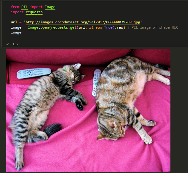

노이즈는 Pilow 이미지가 아닌 Pytorch 텐서에 추가되므로 PIL 이미지를 PyTorch 텐서로 변환합니다. 이미지를 255로 나누어 [0,1] 범위로 변환한 뒤에 n*2 -1 을 도입해 [-1,1]로 변환 가능합니다.

PIL image → Pytorch tensor

from torchvision.transforms import Compose, ToTensor, Lambda, ToPILImage, CenterCrop, Resize

image_size = 128
transform = Compose([
    Resize(image_size),
    CenterCrop(image_size),
    ToTensor(),# turn into torch Tensor of shape CHW, divide by 255
    Lambda(lambda t: (t * 2) - 1),

])

x_start = transform(image).unsqueeze(0)
x_start.shape

Output:
----------------------------------------------------------------------------------------------------
torch.Size([1, 3, 128, 128])

반대 과정도 정의해줍시다

Pytorch tensor → PIL image

import numpy as np

reverse_transform = Compose([
     Lambda(lambda t: (t + 1) / 2),
     Lambda(lambda t: t.permute(1, 2, 0)),# CHW to HWC
     Lambda(lambda t: t * 255.),
     Lambda(lambda t: t.numpy().astype(np.uint8)),
     ToPILImage(),
])

이제 특정 time step에 대해서 test를 하게 되면 아래와 같은 이미지를 볼 수 있습니다.

def get_noisy_image(x_start, t):
	# add noise
    x_noisy = q_sample(x_start, t=t)

    # turn back into PIL image
    noisy_image = reverse_transfrom(x_noisy.squeeze())

    return noisy_image

# take time step
t = torch.tensor([40])
get_noisy_image(x_start, t)

다양한 time step에 대해서 test를 하게 되면 아래와 같은 이미지를 볼 수 있습니다.

import matplotlib.pyplot as plt

# use seed for reproducability
torch.manual_seed(0)

# source: https://pytorch.org/vision/stable/auto_examples/plot_transforms.html#sphx-glr-auto-examples-plot-transforms-pydef plot(imgs, with_orig=False, row_title=None, **imshow_kwargs):
    if not isinstance(imgs[0], list):
# Make a 2d grid even if there's just 1 row
        imgs = [imgs]

    num_rows = len(imgs)
    num_cols = len(imgs[0]) + with_orig
    fig, axs = plt.subplots(figsize=(200,200), nrows=num_rows, ncols=num_cols, squeeze=False)
    for row_idx, row in enumerate(imgs):
        row = [image] + row if with_orig else row
        for col_idx, img in enumerate(row):
            ax = axs[row_idx, col_idx]
            ax.imshow(np.asarray(img), **imshow_kwargs)
            ax.set(xticklabels=[], yticklabels=[], xticks=[], yticks=[])

    if with_orig:
        axs[0, 0].set(title='Original image')
        axs[0, 0].title.set_size(8)
    if row_title is not None:
        for row_idx in range(num_rows):
            axs[row_idx, 0].set(ylabel=row_title[row_idx])

    plt.tight_layout()

Loss Function

손실함수 3종류를 정의한 코드입니다. 손실 함수의 유형은 L1 손실, L2 손실(MSE), 또는 Huber 손실 총 3가지입니다.

def p_losses(denoise_model, x_start, t, noise=None, loss_type="l1"):
    if noise is None:
        noise = torch.randn_like(x_start)

    x_noisy = q_sample(x_start=x_start, t=t, noise=noise)
    predicted_noise = denoise_model(x_noisy, t)

    if loss_type == 'l1':
        loss = F.l1_loss(noise, predicted_noise)
    elif loss_type == 'l2':
        loss = F.mse_loss(noise, predicted_noise)
    elif loss_type == "huber":
        loss = F.smooth_l1_loss(noise, predicted_noise)
    else:
        raise NotImplementedError()

    return loss

Dataset

이제 학습할 데이터셋을 준비해봅시다. 참고한 포스트에서는 mnist 데이터를 통해 진행했지만 저는 celebA 데이터셋을 이용했습니다. 각 이미지는 128*128 사이즈입니다.

import torch
from torch.utils.data import DataLoader
from torchvision import datasets, transforms

# 데이터셋 경로 설정
data_dir = '로컬 경로'

image_size = 128
channels = 3
batch_size = 32

# 데이터 전처리 파이프라인 설정 (이미지 크기 조정 및 정규화)
transform = transforms.Compose([
    transforms.Resize((128, 128)),  # 이미지를 128x128로 크기 조정
    transforms.RandomHorizontalFlip(),  # 랜덤으로 좌우 반전
    transforms.ToTensor(),          # 이미지를 PyTorch 텐서로 변환
    transforms.Normalize([0.5, 0.5, 0.5], [0.5, 0.5, 0.5])  # -1에서 1 범위로 정규화
])

# 기존 ImageFolder에서 데이터를 로드
image_folder_dataset = datasets.ImageFolder(root=data_dir, transform=transform)

# 커스텀 데이터셋 클래스 정의
class CustomDataset(torch.utils.data.Dataset):
    def __init__(self, image_folder_dataset):
        self.dataset = image_folder_dataset

    def __len__(self):
        return len(self.dataset)

    def __getitem__(self, idx):
        image, label = self.dataset[idx]
        # 딕셔너리 형태로 반환
        return {'pixel_values': image}

# 커스텀 데이터셋을 DataLoader로 사용
custom_dataset = CustomDataset(image_folder_dataset)
dataloader = DataLoader(custom_dataset, batch_size=32, shuffle=True, num_workers=4)

# 데이터 확인
batch = next(iter(dataloader))
print(batch.keys())  # dict_keys(['pixel_values', 'label'])
print(f'이미지 배치 크기: {batch["pixel_values"].size()}')  # 예: [16, 3, 128, 128]
print(f'이미지 배치 크기: {batch["pixel_values"].size()}')  # 예: [16, 3, 128, 128]

Sampling

샘플링을 해봅시다. 새로운 이미지를 디퓨전 모델을 통해 생성하는 과정은 앞선 forward diffusion process를 반대로 하는 것과 같습니다.

먼저, T 단계에서 시작하여, 가우시안 분포에서 순수한 노이즈를 샘플링합니다. 그런 다음, 신경망을 사용하여 점진적으로 노이즈를 제거합니다. 이때 신경망은 학습한 조건부 확률( $p(x_{t-1} | x_t)$ )을 이용해 노이즈를 줄여갑니다. 최종적으로 t=0 단계에서 완전히 노이즈가 제거된 이미지에 도달하게 됩니다.

$p(x_{t-1} | x_t) = \mathcal{N}(x_{t-1}; \mu_t(x_t, t), \sigma_t^2 I)$

여기서:

$\mathcal{N}(x_{t-1}; \mu_t(x_t, t), \sigma_t^2 I)$ : 정규분포로, 평균이 $\mu_t$ , 분산이 $\sigma_t^2$ 인 정규분포.
$\mu_t(x_t, t)$ : 신경망이 예측한 평균값으로, 타임스텝 t 에서 t-1 로 이동할 때의 이미지의 상태.
$\sigma_t^2$ : 분산(variance)는 미리 알고 있는 값이며, t에 의존하는 상수입니다.

위에서 설명한 것처럼, 노이즈를 예측해 평균의 재매개변수화를 적용하면, 약간 덜 노이즈가 제거된 $x_{t-1}$ 를 얻을 수 있습니다. 이 과정에서 분산(variance)은 미리 알고 있는 값입니다.

평균 $\mu_t$ 의 재매개변수화 (reparameterization):

평균 $\mu_t(x_t, t)$ 는 노이즈 예측기를 사용하여 다음과 같이 재매개변수화됩니다:

$\mu_t(x_t, t) = \frac{1}{\sqrt{\alpha_t}} \left( x_t - \frac{\beta_t}{\sqrt{1 - \bar{\alpha}t}} \epsilon_\theta(x_t, t) \right)$

여기서:

$\alpha_t$ : 타임스텝 t에 따른 고정된 값.
$\beta_t$ : 타임스텝 t에서의 노이즈 분산.
$\bar{\alpha}_t$ : $\alpha_t$ 의 누적곱.
$\epsilon_\theta(x_t, t)$ : 신경망이 예측한 노이즈 값.

더 자세히 수식에 대해 알고 싶으시다면 해당 포스트를 참고하시면 됩니다.

결과적으로 알고리즘 2의 라인 4는 아래와 같이 정리될 수 있습니다.

$x_{t-1} = \mu_t(x_t, t) + \sigma_t \cdot z$

이를 참고해서 코드를 살펴봅시다.

save_interval = 30

@torch.no_grad()
def p_sample(model, x, t, t_index):
    betas_t = extract(betas, t, x.shape)
    sqrt_one_minus_alphas_cumprod_t = extract(
        sqrt_one_minus_alphas_cumprod, t, x.shape
    )
    sqrt_recip_alphas_t = extract(sqrt_recip_alphas, t, x.shape)
    
    # Equation 11 in the paper
    # Use our model (noise predictor) to predict the mean
    model_mean = sqrt_recip_alphas_t * (
        x - betas_t * model(x, t) / sqrt_one_minus_alphas_cumprod_t
    )

    if t_index == 0:
        return model_mean
    else:
        posterior_variance_t = extract(posterior_variance, t, x.shape)
        noise = torch.randn_like(x)
        # Algorithm 2 line 4:
        return model_mean + torch.sqrt(posterior_variance_t) * noise 

# Algorithm 2 (including returning all images)
@torch.no_grad()
def p_sample_loop(model, shape):
    device = next(model.parameters()).device

    b = shape[0]
    # 순수한 가우시안 노이즈(임의로 생성된 이미지)
    img = torch.randn(shape, device=device)
    imgs = []

    # 각 타임스텝마다 p_sample()을 호출하여 샘플을 생성하고, 그 결과를 imgs 리스트에 저장합니다.
    # 모든 타임스텝이 완료되면, 각 타임스텝에서 생성된 이미지가 리스트에 저장됩니다.
    for i in tqdm(reversed(range(0, timesteps)), desc='sampling loop time step', total=timesteps):
        img = p_sample(model, img, torch.full((b,), i, device=device, dtype=torch.long), i)
        # 특정 간격마다 이미지를 저장
        if i % save_interval == 0:
            imgs.append(img.cpu())
        # imgs.append(img.cpu().numpy())
    return imgs
# 주어진 이미지 크기, 배치 크기, 채널 수에 맞춰서 이미지 생성 루프를 호출합니다.
# 이 함수는 최종적으로 여러 개의 이미지를 반환합니다.
@torch.no_grad()
def sample(model, image_size= image_size, batch_size=batch_size, channels=channels):
    return p_sample_loop(model, shape=(batch_size, channels, image_size, image_size))

→ 샘플링을 이와 같이 할 시에 샘플링 품질이 매우 좋지 않았음

따라서 공식 코드를 참고하여 아래 수식을 구현해줬습니다.

$\tilde{\mu}_t(x_t, x_0) = \frac{\sqrt{\bar{\alpha}_{t-1}} \beta_t}{1 - \bar{\alpha}_t} x_0 + \frac{\sqrt{\alpha_t}(1 - \bar{\alpha}_{t-1})}{1 - \bar{\alpha}_t} x_t$

이때 $x_0$ 은 현재 타임스텝에서의 이미지인 $x_t$ 와 현재 타임스텝에서 모델이 예측한 노이즈인 ϵ을 통해 추정한 이미지입니다. 따라서 $x_0$ 은 아래와 같이 나타낼 수 있습니다.

$x_0 = \frac{x_t}{\sqrt{\bar{\alpha}_t}} - \left(\frac{\sqrt{1 - \bar{\alpha}_t}}{\sqrt{\bar{\alpha}_t}}\right) \epsilon$

이러한 공식을 적용해 수정을 해주게 된다면, 아래와 같이 코드로 나타낼 수 있습니다.

@torch.no_grad()
def p_sample(model, x, t, t_index):
    betas_t = extract(betas, t, x.shape)
    sqrt_one_minus_alphas_cumprod_t = extract(
        sqrt_one_minus_alphas_cumprod, t, x.shape
    )
    
    # 공식 변환 (μ̃t 사용)
    # Equation 변환: μ̃_t(x_t, x_0) = √(ᾱ_t−1)β_t / (1 − ᾱ_t) * x_0 + √(α_t)(1 − ᾱ_t−1) / (1 − ᾱ_t) * x_t
    x_0_pred = model(x, t)  # 모델이 예측한 x_0
    alpha_t = extract(alphas, t, x.shape)
    alpha_cumprod_t_prev = extract(alphas_cumprod_prev, t, x.shape)
    
    # μ̃_t 계산
    model_mean = (
        (torch.sqrt(alpha_cumprod_t_prev) * betas_t / (1 - sqrt_one_minus_alphas_cumprod_t)) * x_0_pred +
        (torch.sqrt(alpha_t) * (1 - alpha_cumprod_t_prev) / (1 - sqrt_one_minus_alphas_cumprod_t)) * x
    )
    
    # 완전히 노이즈가 제거된 최종 이미지
    if t_index == 0:
        return model_mean
    # 노이즈가 제거되지 않은 이미지
    else:
        # posterior의 분산을 추출({σ_t}^2)하고 새로운 가우시안 노이즈를 샘플링하여 추가
        posterior_variance_t = extract(posterior_variance, t, x.shape)
        noise = torch.randn_like(x)
        # Algorithm 2 line 4:
        return model_mean + torch.sqrt(posterior_variance_t) * noise

Train the model

이제 모델을 학습시켜봅시다. 학습 중에 주기적으로 생성된 이미지를 저장하기 위해 아래와 같은 코드를 작성해주었습니다.

from pathlib import Path

def num_to_groups(num, divisor):
    groups = num // divisor
    remainder = num % divisor
    arr = [divisor] * groups
    if remainder > 0:
        arr.append(remainder)
    return arr

results_folder = Path("./results")
results_folder.mkdir(exist_ok = True)
save_and_sample_every = 2000

모델을 정의한 뒤에 GPU로 이동시켜주고, 데이터가 많은 관계로 GPU 병렬처리 해주었습니다.

from torch.optim import Adam

model = Unet(
    dim=image_size,
    channels=channels,
    dim_mults=(1, 2, 4, 8)
)

device = torch.device("cuda" if torch.cuda.is_available() else "cpu")
model = model.to(device)
# 멀티 GPU 설정이 가능한 경우에만 DataParallel 사용
if torch.cuda.device_count() > 1:
    model = torch.nn.DataParallel(model, device_ids=[0,1,2,6])

optimizer = Adam(model.parameters(), lr=1e-3)

학습을 시작해봅시다. 이때 기울기 클리핑과 코사인 스케줄러를 이용해 gradient explosion을 방지했습니다.

from torchvision.utils import save_image
from torch.utils.tensorboard import SummaryWriter
from torch.optim.lr_scheduler import CosineAnnealingLR
import torch
import torch.nn.utils as utils
import os

epochs = 15
save_path = "./checkpoints"  # 모델과 옵티마이저를 저장할 폴더
# TensorBoard writer 생성
writer = SummaryWriter(log_dir="./runs/experiment_3")  # 로그 파일이 저장될 경로

# CosineAnnealingLR 스케줄러 정의 (optimizer와 epochs에 맞춰서 설정)
scheduler = CosineAnnealingLR(optimizer, T_max=epochs, eta_min=0)

# Create the directory if it doesn't exist
import os
if not os.path.exists(save_path):
    os.makedirs(save_path)

for epoch in tqdm(range(epochs), desc="epoch"):
    print(f"Epoch: {epoch}")
    for step, batch in enumerate(dataloader):
      optimizer.zero_grad()

      batch_size = batch["pixel_values"].shape[0]
      batch = batch["pixel_values"].to(device)

      # Algorithm 1 line 3: sample t uniformally for every example in the batch
      t = torch.randint(0, timesteps, (batch_size,), device=device).long()

      loss = p_losses(model, batch, t, loss_type="l2")

      if step % 100 == 0:
        print(f"Step {step} - Loss: {loss.item()}")
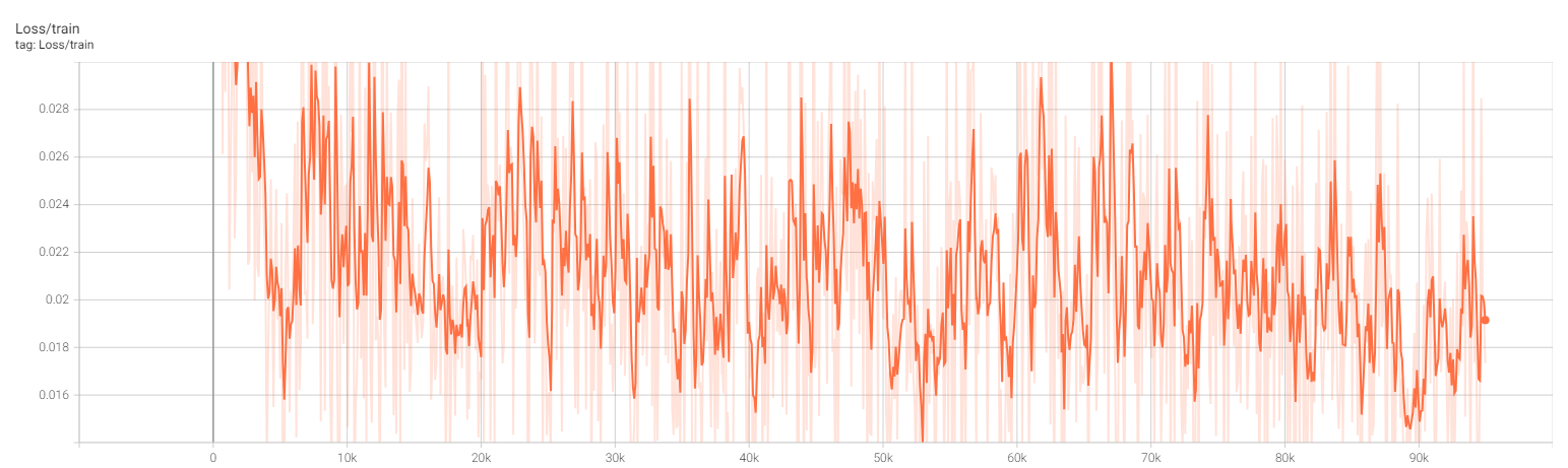
        writer.add_scalar("Loss/train", loss.item(), epoch * len(dataloader) + step)  # TensorBoard에 손실 기록

      loss.backward()

       # 기울기 클리핑 적용 (L2 노름)
      max_grad_norm = 1.0  # 원하는 최대 기울기 노름 설정
      utils.clip_grad_norm_(model.parameters(), max_grad_norm)
      
      optimizer.step()

      # 스케줄러로 학습률 업데이트
      scheduler.step()

      # save generated images
      if step != 0 and step % save_and_sample_every == 0:
        milestone = step // save_and_sample_every
        batches = num_to_groups(4, batch_size)

        all_images_list = list(map(lambda n: sample(model, batch_size=n, channels=channels), batches))
        all_images = torch.cat(all_images_list[0], dim=0)
        all_images = (all_images + 1) * 0.5 # [-1, 1] 범위를 갖는 이미지를 [0, 1] 범위로 정규화

        # Save generated images to TensorBoard
        writer.add_images(f"Generated Images/epoch_{epoch}_step_{step}", all_images, epoch * len(dataloader) + step)
        step_num = step + epoch * 6000
        save_image(all_images, str(results_folder / f'sample-{step_num}.png'), nrow = 8)

    # epoch마다 모델과 옵티마이저 저장
    torch.save({
        'epoch': epoch,
        'model_state_dict': model.state_dict(),
        'optimizer_state_dict': optimizer.state_dict(),
        'loss': loss.item()
    }, os.path.join(save_path, f"model_epoch_{epoch}.pt"))

    print(f"Model saved for epoch {epoch}")