References
PRIORITIZED EXPERIENCE REPLAY (2016, ICLR)
Importance Sampling in DRL

Prioritized Experience Replay

기존 Deep Q Network(DQN)의 replay buffer에서는 buffer에 저장되어 있던 experience transitions들을 uniformly sampling 했다. 이는 개별 transition의 중요성을 반영하지 못한다. PER에서는 중요한 transition을 더많이 replay 해서 학습의 효율의 향상시키고자 한다.

Prioritizing with TD-Error

개별 transition에 대한 priority를 부여할 때 이상적인 값은 RL agent가 현재 state에서 어떤 transition으로부터 얼마나 배울 수 있는가 이다. 하지만 이는 직접적으로 구할 수 없다. 이때 TD-error($\delta$)의 크기는 해당 지표의 합리적인 대체값이 될 수 있다. 이는 아래와 같이 정의된다:

Greedy TD-error prioritization

Greedy TD-error prioritization 방법에서는 아래와 같은 순서로 transition에 대한 prioritization과 sampling이 진행된다.

1. 매 transition마다 TD-Error를 계산해서 replay memory에 저장. 이때 처음 관측되는 transition에 대해서는 maximum priority를 적용한다 → 최소한 1번이상의 sampling을 보장.
2. TD error가 가장 큰 transition을 sampling
3. Sampling된 transition을 이용해서 network update

이러한 greedy TD-error prioritization에는 아래와 같은 몇가지 문제점이 있다.

1. TD-error가 replay된 transition에 대해서만 update된다.
2. noise에 취약(e.g. reward가 stochastic한 경우)하며 이는 bootstrapping환경에서 더욱 심해진다. → 잘못된 근사가 또 다른 노이즈의 근원이 된다.
3. 학습시 경험의 일부에만 초점을 맞춘다. 특히 function approximation시에 (e.g. DNN) 오차가 천천히 줄어들기 때문에 초기에 오차가 컷던 transition들이 빈번하게 재학습되며 이는 over-fitting되기 쉬운 환경을 조성한다.

Stochastic Sampling Method

Greedy TD-error prioritization method의 단점을 보완하기 위해 PRIORITIZED EXPERIENCE REPLAY에서는 stochastic sampling method를 제안한다. Stochastic sampling method에서는 각 transition의 sampling확률이 $|\delta|$에 대해 단조성을 띄게 함과 동시에 최하위 priority의 transition에 대해서도 0이 아닌 sampling 확률을 보장한다. Transition $i$의 sampling확률은 다음과 같다:

이때 $p_i = |\delta_t|+\epsilon$으로 정의되며 sample $i$의 중요도 이다. $\epsilon$은 모든 transition에 대하여 일괄적으로 더해지는 값으로서 $P(i)\neq 0$임을 보장한다. $\alpha$는 sampling시에 $p_i$를 반영하는 정도로서 0과 1사이의 값으로 정의되며, $\alpha = 0$일 때는 uniformly sampling과 동일하다. $p_i$를 계산하는 또다른 방법으로는 $|\delta|$값 크기에 따른 순위를 기반으로 한 방법도 있다. 이를 rank-based prioritization 이라고 하며 $p_i=\frac{1}{rank(i)}$와 같이 계산된다.

Annealing The Bias with Importance Sampling (IS)

Stochastic update시에 sampling의 분포는 기댓값 대상이 되는 분포와 동일한 분포를 따른다는 점을 전제로 한다. 하지만 PER에서는 본래의 기댓값의 대상이 되는 함수가 따르는 분포가 아닌 다른 분포에서의 sampling을 통하여 원하는 값을 얻고자 한다. 이 처럼 본래 $x$가 따르는 분포인 $p(x)$가 아닌 다른 분포 $q(x)$에서 $\mathbb{E}_{x\sim p}[f(x)]$의 값을 추정하는 방법을 Importance Sampling(IS)(Importnace Sampling 추가자료) 이라고 한다. 이러한 sampling 분포의 변화는 모델이 priority가 높은 transition에 대한 loss의 기대값으로 수렴하게 되는 현상을 발생시키는데 이러한 bias를 가중치 update시에 IS weight($w_i$)를 곱해줌으로서 보정해준다 :

해당 IS weight는 항상 가중치가 업데이트 값을 축소하는 방향으로 작용하게끔 하기위해 $\frac{1}{\max_iw_i}$로 정규화 된다. 즉, 최종 IS weight는 $w_i =\frac{(N\cdot P(i))^{-\beta}}{\max_iw_i}$와 같다.

We can correct this bias by using importance-sampling (IS) weights that fully compensates for the non-uniform probabilities $P(i)$ if $β = 1$. These weights can be folded into the Q-learning update by using $w_iδ_i$ instead of $δ_i$. For stability reasons, we always normalize weights by $\frac{1}{\max_i w_i}$ so that they only scale the update downwards.

— PRIORITIZED EXPERIENCE REPLAY (ICLR, 2016)

위 논문 본문을 보면 using $w_i\delta_i$ instead of $\delta$라고 되어 있는데 이는 loss계산시에 $\mathcal{L}=\frac{1}{2}\delta^2$와 같이 loss가 정의될 때 $\mathcal{L}=\frac{1}{2}(w\cdot\delta)^2$과 같은 형태로 사용하는 것으로 오해할 수 있는데 이게 아니라 최종 loss value에 IS weight $w$가 곱해지는 형태로 $w\cdot \mathcal{L}=\frac{1}{2}\cdot w\cdot \delta^2$과 같이 사용된다. 본문에서 왜 using $w_i\delta_i$ instead of $\delta$와 같이 표현했는지는 아래 식을 통해 알 수 있다($\eta$: learning rate).

• 기존 Q-learning update

• 새로운 Q-learning update 식

• 만약 $\mathcal{L}(\theta) = \frac{1}{2}(w \cdot \delta)^2$으로 둘 경우

이러한 priority baes sampling과 Importance sampling(IS)기반의 보정기법을 통해서 높은 td-error를 가지는 transition들은 자주 샘플링되며 여러번 경험하도록 보장하는 동시에, IS correction을 통해 sampling된 transition의 td-error에 비례하여 gradient magnitude를 줄여준다. 해당 방법을 통해 중요한 transition을 여러번 겪으면서 잘게 쪼개진 step으로 여러번 gradient를 update하며 Taylor Expansion을 재근사 하면서 높은 곡률을 가지는 비선형 함수를 잘 근사하도록 한다.

Atari Experiments and Hyperparameters($\alpha, \beta)$

Atari game 성능 지표로 normalized score를 사용하고 이는 사람보다 얼마나 더 좋은 성과를 내었는가를 나타낸다:

아래의 Figure1, Figure2에서 알 수 있듯이 Priority 기반 sampling이 기존 uniformly sampling보다 좋은 성능을 냄을 알 수 있다. 또한 proportional prioritization이 rank-based prioritization보다 더 뛰어난 성능과 안정성을 보인다.

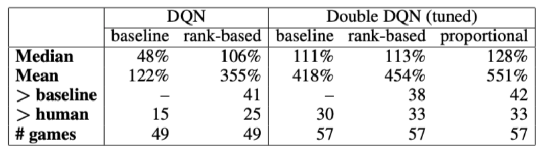[Table1] Summary of normalized scores.

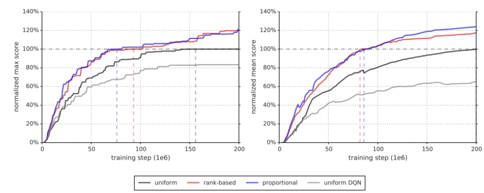[Figure 1] Summary of learning speed.

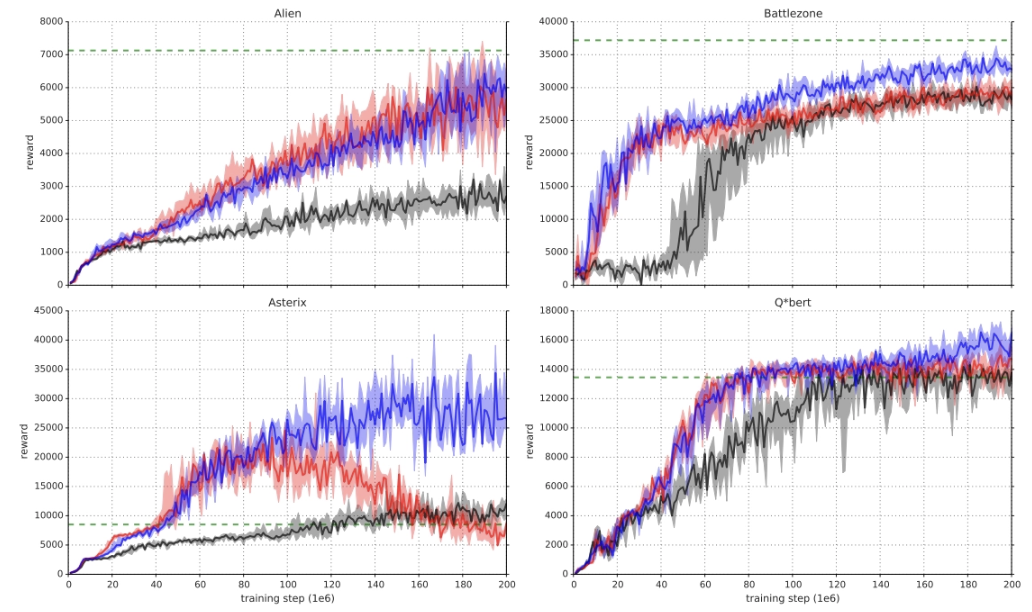[Figure 2] Detailed learning curves for rank-based(red) and proportional(blue) prioritization, uniform DQN baseline(black) and human(dotted line)

개별 Transition의 sampling 확률에 관여하는 $\alpha$값과 Importance Sampling weight을 통한 bias 보정 강도에 관여하는 $\beta$값은 모든 실험에 대해서 고정적으로 사용되었다. $\alpha$같은 경우에는 $0.7$과 $0.6$을 고정값으로 사용했고, $\beta$값은 rank-based같은 경우에는 $0.5$에서 $1$로, proportional variant에서는 $0.4$에서 $1$로 선형으로 annealing한다. 본인의 PER을 적용한 다른 연구에서 $\alpha$값과 $\beta$값을 PER 원논문에서 사용한 값과 동일하게 사용했을 때 좋은 결과를 얻을 수 있었다. PER을 적용할 때 해당 값들을 그대로 사용하거나 아니면 baseline으로 두고 더 좋은 값을 찾아가는 방법을 추천한다.

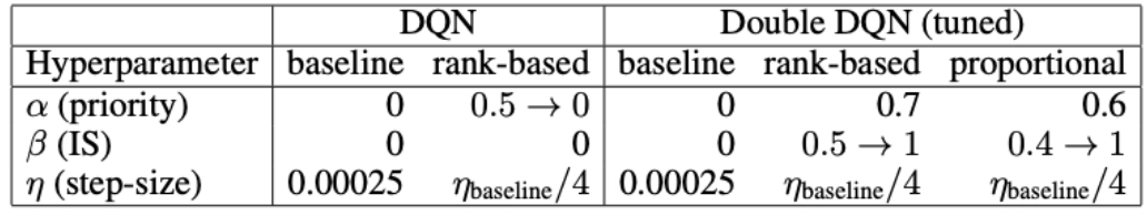[Table 3] Chosen hyperparameters for prioritized variants.

Implementation (Proportional prioritization)

앞선 실험에서 뛰어난 성능을 확인할 수 있었던 proportional prioritization을 위한 Prioritized Replay Buffer를 구현해 보자.

Implementation Sum-tree for PER

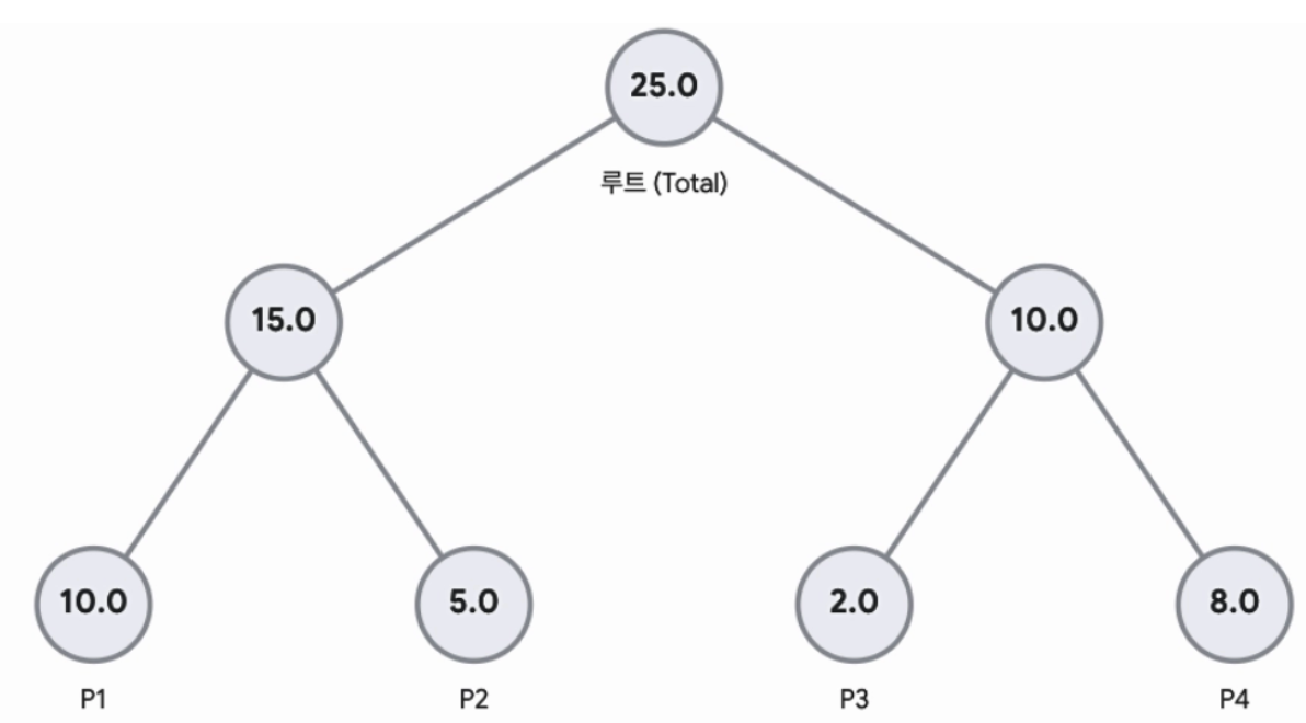
List의 형태로 구현했던 기존 experience replay buffer와는 다르게 PER에서는 sum-tree를 이용하여 buffer를 구현하며 이는 binary heap과 유사하다. Sum-tree의 모든 parent node는 두 child node 값의 합이 되며 각 leaf node는 개별 transition의 priority값($p_i=|\delta_i|+\epsilon)$을 갖는다. Root node는 모든 priority값의 합인 $p_\text{total}$을 갖게된다. List를 사용했을 때 priority값을 update할 때 $O(N)$의 계산시간이 필요했다면, sum-tree는 $O(\log N)$의 시간복잡도를 보장한다.

100만개의 데이터가 List의 형태로 있을 때 어떤 transition하나의 priority값이 바뀌면 총합과 누적합을 다시 구하기 위해 100만 번($O(N)$)의 계산이 필요하다. Sum-Tree를 사용하면 leaf node하나의 값이 바뀌었을 때 트리를 타고 루트까지 올라가며 부모 노드들만 수정하면 되므로 20번 ($O(\log N)$)의 연산만으로 끝난다.

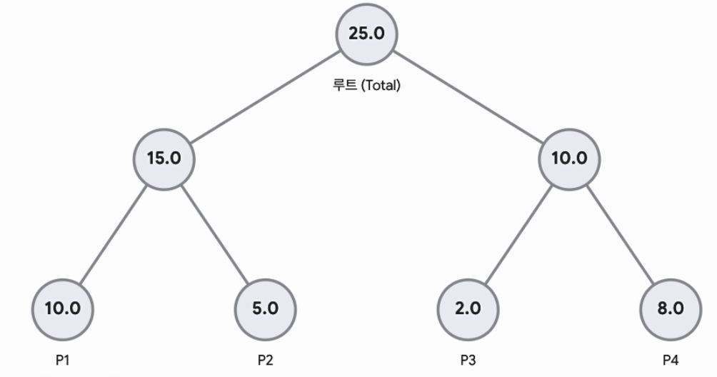[Figure 3] Sum-tree

Batch size가 $k$인 Mini-batch gradient descent를 할 때 다음과 같은 순서로 sampling을 한다.

1. 전체 누적 우선순위 $[0,p_\text{total}]$범위를 $k$등분한다.
2. 각 구간안에서 무작위 난수 값을 뽑는다.
3. 2번에서 뽑은 값이 가리키는 위치에 해당하는 데이터(transition)를 트리에서 찾아서 가져온다.

2번과정에서 뽑은 값을 이용해서 3번 과정을 수행하며 트리를 타고 내려갈 때 항상 현재 노드에서 왼쪽 자식 노드값을 확인한다.

이를 Figure 3으로 예시를 들어보면 아래와 같다. Batch size =2라고 하자.

1. $[0,25]$를 2개의 구간으로 나눈다. $[0,12]$, $[13,25]$
2. $[0,12]$범위에서 하나, $[13,25]$범위에서 하나 총 2개의 난수를 뽑는다.
3. $[0,12]$에서 9가 뽑히고 $[13,25]$에서 21이 뽑혔다고 가정해보자 그럼 각각 $\text{P1}$과 $\text{P4}$가 sampling되는데 뽑히는 원리는 아래와 같다.

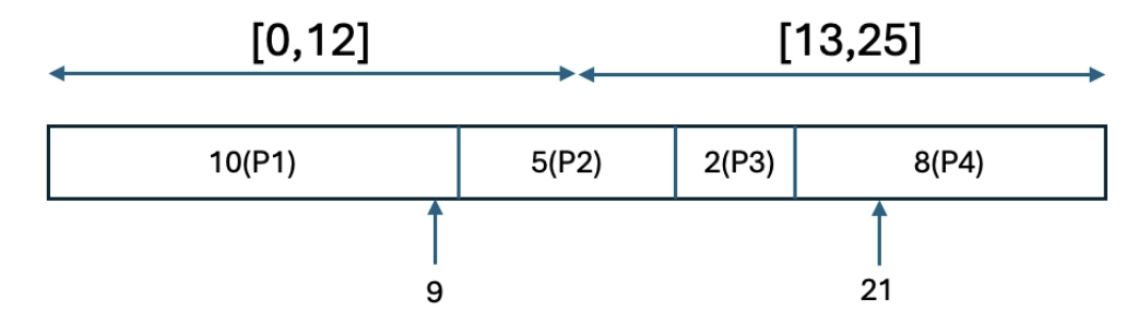[Figure 4] Transition sampling process.

PER구현을 위한 sum-tree 코드는 아래와 같다

Code1. sum-tree code for PER

import numpy as np
import random

class SumTree:
    def __init__(self, capacity):
        self.capacity = capacity
        self.tree = np.zeros(2 * capacity - 1)    
        self.data = np.zeros(capacity, dtype=object)    
        self.write = 0 
        self.n_entries = 0

    def _propagate(self, idx, change):
        while idx != 0:
            idx = (idx - 1) // 2
            self.tree[idx] += change
        
    def _retrieve(self, idx, s) -> int:
        left = 2 * idx + 1     
        right = left + 1

        if left >= len(self.tree):
            return idx 
        
        if s <= self.tree[left]:
            return self._retrieve(left, s)
        else:
            return self._retrieve(right, s - self.tree[left])
    
    def total_priority(self):
        return self.tree[0]

    
    def update(self, idx, p):
        change = p - self.tree[idx]
        self.tree[idx] = p
        self._propagate(idx, change=change)
    
    def add(self, p, data):
        idx = self.write + self.capacity - 1 
        self.data[self.write] = data
        self.update(idx, p)

        self.write += 1
        if self.write >= self.capacity:
            self.write = 0
        if self.n_entries < self.capacity:
            self.n_entries += 1
    
    def get(self, s):
        idx = self._retrieve(0, s)          
        data_idx = idx - self.capacity + 1      

        return (idx, self.tree[idx], self.data[data_idx])

위 코드에서 알 수 있듯이 buffer capacity가 $N$일 때, sum-tree가 가지는 전체 node 수는 $2N-1$개이다. self.tree 는 개별 transition의 priority들이 저장되는 sum-tree로서, 해당 값들은 leaf node에 저장되어 있고 각각의 parent node들은 priority의 부분합에 관한 정보를 담고 있다. self.data 에 실제 개별 transition들의 정보가 담겨 있다. 개별 transition은 $(s,a, r,s')$ 와 같은형태로 저장되어 있다.

Implementation of PER

Code1을 이용한 Prioritized Replay Buffer code는 아래와 같다.

Code2. PER buffer code

import numpy as np
from typing import Tuple, List
import random
import torch
from sumtree import SumTree    # code1

class PrioritizedReplayBuffer:
    def __init__(self, capacity: int, alpha=0.6):
        self.tree = SumTree(capacity=capacity)
        self.alpha = alpha
        self.max_priority = 1.0 
        

    def push(self, state: Tuple[float], action: List[int], reward: float, next_state: Tuple[float], done: bool):
        data = (state, action, reward, next_state, done)
        p = self.max_priority 
        self.tree.add(p=p, data=data)

    def sample(self, batch_size, beta, device="cpu"):
        batch_idx, batch_priorities = [], []
        batch_data = []
        segment = self.tree.total_priority() / batch_size

        for i in range(batch_size):
            a = segment * i
            b = segment * (i + 1)
            s = random.uniform(a, b)

            idx, p, data = self.tree.get(s)
            batch_idx.append(idx)
            batch_priorities.append(p)
            batch_data.append(data)
        
        state, action, reward, next_state, done = zip(*batch_data)

        sampling_probabilities = np.array(batch_priorities) / self.tree.total_priority()
        is_weights = np.power(self.tree.n_entries * sampling_probabilities, -beta)
        is_weights /= is_weights.max()

        return (
            torch.as_tensor(np.array(state), dtype=torch.float32, device=device),
            torch.as_tensor(np.array(action), dtype=torch.long, device=device),
            torch.as_tensor(np.array(reward), dtype=torch.float32, device=device),
            torch.as_tensor(np.array(next_state), dtype=torch.float32, device=device),
            torch.as_tensor(np.array(done), dtype=torch.bool, device=device),

            torch.as_tensor(np.array(is_weights), dtype=torch.float32, device=device),
            batch_idx
        )
    

    def batch_update(self, tree_idx, abs_errors):
        abs_errors += 1e-5
        ps = np.power(abs_errors, self.alpha)

        for ti, p in zip(tree_idx, ps):
            self.tree.update(ti, p)
            self.max_priority = max(self.max_priority, p)

위 코드를 보면 PER본문에서 설명한 내용들이 전부 반영되어 있는 것을 볼 수 있다. 구체적으로 batch_update() 메서드에서는 수식 $(2)$에 따라 $\alpha$가 반영된 $p_i^\alpha$값이 계산되어 SumTree 에 update된다. 또한, sample() 메서드에서는 각 transition에 대해 수식 $(3)$을 계산한 뒤, 이를 $\max_iw_i$로 정규화한 IS weight를 DRL agent에게 반환하고 있으며, 동일한 메서드 내의 transition sampling 과정을 보면, 직전 sum-tree 구현 파트에서 설명한 transition sampling process가 그대로 구현되어 있음을 알 수 있다. PER을 적용하면서 기존 학습 코드와 비교했을 때 몇가지 부분에 변화가 생긴다.

code3. Changes to training code for PER implementation

# Train without PER
q_network.train()

states, actions, rewards, next_states, dones = replay_buffer.sample(batch_size=batch_size)

q_values = q_network(states)
q_value = q_values.gather(1, actions.unsqueeze(1)).squeeze(1)

with torch.no_grad():
    next_q_values = target_network(next_states)
    max_next_q = next_q_values.max(1)[0]
    target_q = rewards + gamma * max_next_q * (1 - dones)

optimizer.zero_grad()
loss = criterion_mse(q_value, target_q)
loss.backward()
optimizer.step()




# Train with PER
q_network.train()

beta = min(beta_end, beta_start + (beta_end - beta_start) * (global_step / total_steps))
states, actions, rewards, next_states, dones, is_weights, tree_idx = replay_buffer.sample(
    batch_size=batch_size, beta=beta, device=device
)

q_values = q_network(states)    
q_value = q_values.gather(1, actions.unsqueeze(1)).squeeze(1) 

with torch.no_grad():
    next_q_values = target_network(next_states)     
    max_next_q = next_q_values.max(1)[0]            
    target_q = rewards + gamma * max_next_q * (1 - dones)
   
td_errors = torch.abs(target_q - q_value)   # for update priority

optimizer.zero_grad()
raw_loss = criterion_mse(q_value, target_q)  
loss = torch.mean(is_weights * raw_loss)     
loss.backward()
optimizer.step()

replay_buffer.batch_update(tree_idx, td_errors.detach().cpu().numpy())  # update priority

code를 보면 IS weight계산을 위한 $\beta$값 update를 위한 코드가 추가 된 것을 볼 수 있고, sampling시에 is_weights와 priority update를 위한 tree_idx 를 추가로 전달받으며, 이를 이용한 priority update 코드를 마지막 줄에서 확인할 수 있다. 가중치 update 시에도 기존 loss값을 그대로 쓰던 것과는 달리 loss = torch.mean(is_weights * raw_loss) 를 통해 IS weight를 적용하여 최종 loss값을 계산한다.

Appendix

Priority base sampling with IS weight

신경망에서 파라미터를 update할 때, update식은 1차 taylor expansion을 기반으로 하며 아래와 같다.

• Taylor Expansion

• 1st Taylor Expansion

• Loss value update equation.

Loss값을 토대로 가중치를 업데이트할 때 1st taylor expansion의 의존하여 update한다. 즉, $\mathcal{L}(\theta)$부근이 $\mathcal{L}(\theta) + \nabla_\theta\mathcal{L}(\theta) \cdot \Delta\theta$형태의 직선이라고 가정하고 $\theta$를 update한다. 이때 아래 사진에서도 볼 수 있듯이 큰 step으로 이동할 때 실제 Loss값과의 오차가 급격하게 벌어지는 것을 볼 수 있다. 큰 update step을 가질 때 실제 loss값 과의 오차 정도는 함수의 곡률이 커질 수록 더 심해진다. PER에서는 IS correction을 통해서 td-error가 큰 transition에 대한 gradient magnitude를 줄여놓고 priority base sampling을 통해 이를 자주 뽑아주면서 큰 곡률을 가지는 비선형함수에서도 안정적으로 loss값을 근사하며 가중치를 update할 수 있다. 이를 논문 본문에서는 다음과 같이 표현한다.

In our approach instead, prioritization makes sure high-error transitions are seen many times, while the IS correction reduces the gradient magnitudes (and thus the effective step size in parameter space), and allowing the algorithm follow the curvature of highly
non-linear optimization landscapes because the Taylor expansion is constantly re-approximated.

— PRIORITIZED EXPERIENCE REPLAY (ICLR, 2016)

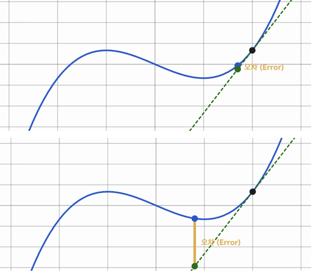[Figure 5] Difference in approximation error based on update steps in the nonlinear optimization space